36 Lifelong Learning: How the Brain Avoids Forgetting
Learning Objectives By the end of this chapter, you will be able to:
- Understand the “stability-plasticity dilemma” as a fundamental challenge for any learning system.
- Explain why standard deep learning models suffer from “catastrophic forgetting.”
- Analyze the brain’s elegant, two-part solution to this dilemma involving the hippocampus and neocortex.
- Compare the main computational approaches to continual learning in AI, such as replay and regularization.
- Connect these AI techniques to their direct neuroscientific inspirations.
36.1 26.1 The Stability-Plasticity Dilemma
A hallmark of intelligence is the ability to learn continuously from an endless stream of experience. Humans and animals do this effortlessly. We learn new skills, facts, and faces throughout our lives without erasing the old ones. This capacity for lifelong learning is a fundamental challenge for artificial intelligence.
AI models face a core trade-off known as the stability-plasticity dilemma: - Plasticity: The ability to rapidly learn new information. - Stability: The ability to retain old knowledge without it being corrupted by new learning.
If a system is too plastic, new information will constantly overwrite old memories. If it’s too stable, it becomes rigid and unable to learn anything new. Modern deep learning models are extremely plastic, which leads to a catastrophic failure mode.
26.1.1 The Problem: Catastrophic Forgetting
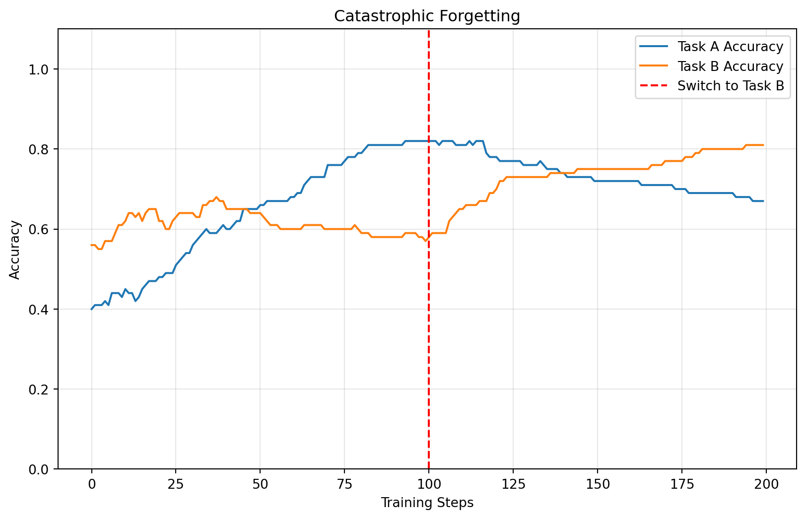
When a standard neural network is trained on a new task, it overwrites the synaptic weights that encoded the knowledge of previous tasks. The new learning catastrophically interferes with and destroys the old.
Imagine training an AI to first recognize cats, and then training it to recognize dogs. After learning to identify dogs, it will likely have forgotten how to recognize cats entirely. Its performance on the first task drops to near zero. This is catastrophic forgetting, and it is the single biggest barrier to creating AI that can learn and adapt in the real world.
36.2 26.2 The Brain’s Solution: Complementary Learning Systems
How does the brain solve the stability-plasticity dilemma? It uses a brilliant architectural solution: complementary learning systems. The brain has two different, interconnected memory systems that learn at different rates.
The Sculptor And The Library Analogy Imagine a sculptor and a grand library working together.
The Hippocampus (The Sculptor’s Studio): This is a fast, messy, creative space. The sculptor (the hippocampus) takes new experiences (lumps of clay) and rapidly shapes them into detailed, specific memories (individual sculptures). The studio is highly plastic—it’s easy to make new sculptures. But it’s also small and temporary.
The Neocortex (The Grand Library): This is a vast, organized, and permanent archive. The librarian (the neocortex) is very slow and careful. It doesn’t accept every new sculpture from the studio.
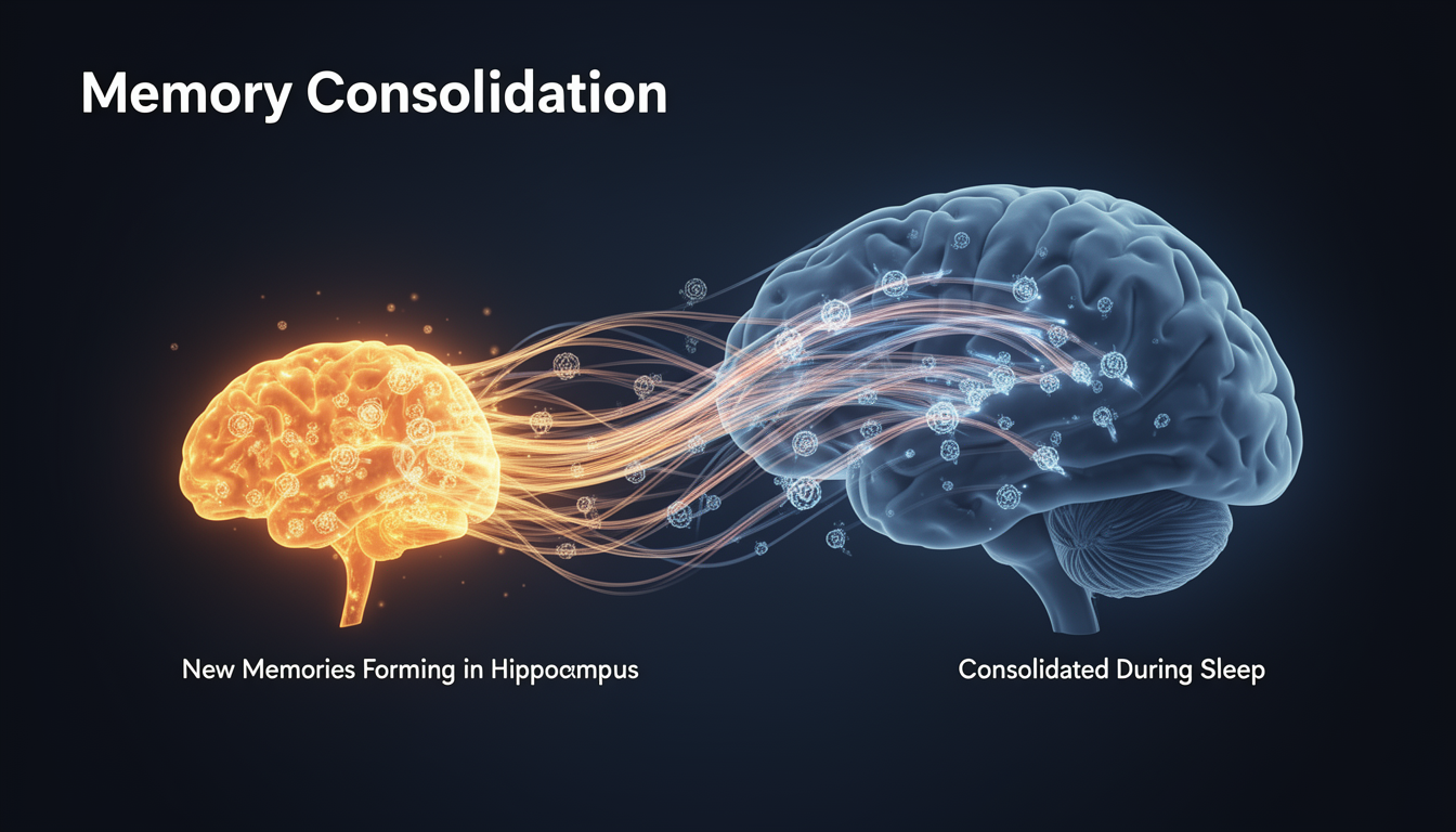
Memory Consolidation (The Nightly Review): During sleep, the librarian reviews the most important sculptures created that day. It then painstakingly casts them in marble and moves them into the grand library, integrating them with the existing collection. This process is slow and deliberate, ensuring the library remains stable and organized.
This two-part system gets the best of both worlds: fast, flexible learning in the studio, and slow, stable integration in the library.
This is precisely what happens in the brain. The hippocampus rapidly encodes new episodic memories. Then, during sleep, the brain engages in memory replay, reactivating these hippocampal traces and gradually training the neocortex to integrate this new information into its long-term, stable knowledge base.
36.3 26.3 Elastic Weight Consolidation (EWC): Full Derivation
Inspired by the brain’s complementary learning systems, AI researchers have developed several families of techniques for continual learning. We begin with one of the most influential: Elastic Weight Consolidation (EWC), which provides a principled mathematical framework for protecting important knowledge while remaining plastic to new information.
26.3.1 The Core Intuition
The key insight behind EWC is that not all weights in a neural network are equally important for a given task. Some weights are critical for maintaining good performance, while others can be changed freely without affecting the learned knowledge. EWC identifies the important weights and then protects them from large changes when learning new tasks.
This is directly inspired by synaptic consolidation in the brain, where important synapses become more stable and resistant to modification over time. The challenge is: how do we measure which weights are “important”?
26.3.2 Mathematical Formulation
After training a neural network on task \(A\), we have learned optimal parameters \(\theta^*_A\). When we now train on task \(B\), we want to find parameters \(\theta^*_B\) that perform well on task \(B\) while staying close to \(\theta^*_A\) for task \(A\).
From a Bayesian perspective, we want to find parameters that maximize the posterior probability:
\[ \log p(\theta | \mathcal{D}) = \log p(\mathcal{D}_B | \theta) + \log p(\theta | \mathcal{D}_A) - \log p(\mathcal{D}_B) \]
where \(\mathcal{D}_A\) and \(\mathcal{D}_B\) are the datasets for tasks \(A\) and \(B\). The first term is the log-likelihood of the new data, and the second term is our prior, conditioned on the old data.
The key approximation in EWC is to approximate the posterior \(p(\theta | \mathcal{D}_A)\) as a Gaussian distribution centered at \(\theta^*_A\):
\[ \log p(\theta | \mathcal{D}_A) \approx \log p(\theta^*_A | \mathcal{D}_A) - \frac{1}{2} \sum_i F_i (\theta_i - \theta^*_{A,i})^2 \]
where \(F_i\) is the Fisher Information Matrix diagonal element for parameter \(i\). The Fisher Information Matrix measures the curvature of the loss landscape around \(\theta^*_A\)—parameters with high Fisher information are in steep valleys and are thus important for task \(A\).
26.3.3 The Fisher Information Matrix
The Fisher Information Matrix is defined as:
\[ F_i = \mathbb{E}_{x \sim \mathcal{D}_A} \left[ \left( \frac{\partial \log p(y|x, \theta^*_A)}{\partial \theta_i} \right)^2 \right] \]
In practice, we compute this using samples from the training data:
\[ F_i \approx \frac{1}{N} \sum_{n=1}^{N} \left( \frac{\partial \log p(y_n|x_n, \theta^*_A)}{\partial \theta_i} \right)^2 \]
This tells us how sensitive the model’s predictions are to changes in each parameter. High Fisher information means that changing that parameter would significantly alter the output distribution, making it important to protect.
26.3.4 The EWC Loss Function
Combining these insights, the loss function for learning task \(B\) becomes:
\[ \mathcal{L}(\theta) = \mathcal{L}_B(\theta) + \frac{\lambda}{2} \sum_i F_i (\theta_i - \theta^*_{A,i})^2 \]
where: - \(\mathcal{L}_B(\theta)\) is the standard loss for task \(B\) - The second term is the regularization penalty that prevents important weights from changing - \(\lambda\) is a hyperparameter controlling the strength of regularization
This loss function creates an “elastic” constraint: weights can move, but important weights (high \(F_i\)) are anchored to their old values with strong springs.
26.3.5 Algorithm: EWC Step-by-Step
EWC implementation loaded. Key insight:
- Compute Fisher Information to identify important weights
- Add quadratic penalty to prevent important weights from changing
- Lambda parameter controls rigidity vs plasticity trade-off
26.3.6 Computational Considerations
Memory Requirements: EWC requires storing: - Old optimal parameters \(\theta^*_A\) (same size as model) - Fisher Information Matrix \(F\) (same size as model) - For \(T\) tasks, memory scales as \(O(2T \times |\theta|)\)
Computational Cost: - Computing Fisher Information requires a forward-backward pass over the old dataset - During training on new tasks, computing the penalty adds negligible overhead - Much cheaper than storing and replaying old data
Hyperparameter Tuning: - \(\lambda\) too small: insufficient protection, forgetting occurs - \(\lambda\) too large: too rigid, cannot learn new tasks - Typical range: \(\lambda \in [100, 10000]\) depending on task similarity - Can be adapted per task: \(\lambda_t = \lambda_0 \sqrt{t}\) for \(t\) tasks
26.3.7 Limitations and Extensions
Limitations: 1. Approximations: Diagonal Fisher is only an approximation; full Fisher is too expensive to compute 2. Task Interference: If tasks are very different, even EWC cannot prevent all forgetting 3. Memory Growth: Fisher matrices accumulate linearly with tasks 4. Local Optima: Fisher is computed at a single point \(\theta^*_A\), not capturing the full loss landscape
Extensions: - Online EWC: Update Fisher information incrementally as new data arrives - Synaptic Intelligence: Compute importance based on path integral of parameter gradients during training - Memory Aware Synapses (MAS): Compute importance based on sensitivity of output (not loss) to parameter changes
36.4 26.4 Progressive Neural Networks
While EWC protects old knowledge through regularization, Progressive Neural Networks take a radically different approach: they prevent forgetting by preventing any change to old parameters at all. Instead of trying to find parameters that work for all tasks, they allocate new network capacity for each new task.
26.4.1 Architecture with Lateral Connections
Progressive Neural Networks consist of multiple “columns,” where each column is a separate neural network dedicated to a specific task. The key innovation is the lateral connections that allow new columns to leverage features learned by old columns.
For a network with \(L\) layers learning task \(k\), the hidden activation at layer \(l\) is:
\[ h^{(k)}_l = f\left( W^{(k)}_l h^{(k)}_{l-1} + \sum_{i<k} U^{(k,i)}_l h^{(i)}_{l-1} \right) \]
where: - \(W^{(k)}_l\) are the standard within-column weights - \(U^{(k,i)}_l\) are the lateral adapter weights from column \(i\) to column \(k\) - \(h^{(i)}_{l-1}\) is the hidden activation from previous column \(i\) at layer \(l-1\)
This architecture allows task \(k\) to build upon features learned by all previous tasks \(i < k\), enabling positive forward transfer without any risk of catastrophic forgetting.
Progressive Neural Networks Architecture:
==========================================
 - Task 0 added:
  - Total columns: 1
  - Frozen columns: 0
  - Trainable columns: 1 (column 0)
  - Trainable parameters: 682 / 682
 - Task 1 added:
  - Total columns: 2
  - Frozen columns: 1
  - Trainable columns: 1 (column 1)
  - Trainable parameters: 682 / 1364
 - Task 2 added:
  - Total columns: 3
  - Frozen columns: 2
  - Trainable columns: 1 (column 2)
  - Trainable parameters: 682 / 2046
 - Task 0 output shape: torch.Size([5, 2])
 - Task 1 output shape: torch.Size([5, 2])
 - Task 2 output shape: torch.Size([5, 2])
26.4.2 Transfer Learning Without Forgetting
The beauty of Progressive Networks is that they achieve perfect retention of old tasks (zero forgetting) while simultaneously enabling positive forward transfer to new tasks through lateral connections.
Forward Transfer: New tasks can leverage rich features learned by earlier tasks. For example: - If Task 1 learned edge detectors, Task 2 can reuse them for object recognition - If Task 1 learned to grasp objects, Task 2 can reuse the motor skills for stacking
Backward Transfer: Unlike methods that update shared parameters, Progressive Networks have zero backward transfer (no improvement to old tasks). This is the price of perfect stability.
26.4.3 When to Allocate New Columns
A key design question is: when should we allocate a new column versus continuing to train an existing one?
Strategies: 1. One column per task: Simple and guarantees zero forgetting, but grows linearly with tasks 2. Detect task change: Monitor performance; allocate new column when performance drops 3. Measure task similarity: Use distance metrics (e.g., gradient similarity) to decide if a task is similar enough to share a column 4. Hybrid approach: Allow limited fine-tuning of old columns with EWC-style regularization
Practical Considerations: - Memory grows linearly with number of tasks: \(O(T \times |\theta|)\) - Inference cost also grows: must evaluate all previous columns for lateral connections - Best suited for scenarios with a moderate number of diverse tasks (10-100)
26.4.4 Comparison to Fine-Tuning
| Method | Forgetting | Forward Transfer | Memory | Inference Cost |
|---|---|---|---|---|
| Fine-tuning | High | High | \(O(1)\) | \(O(1)\) |
| Progressive Nets | Zero | High | \(O(T)\) | \(O(T)\) |
| EWC | Low | Medium | \(O(T)\) | \(O(1)\) |
Progressive Networks trade memory and computation for perfect retention and strong transfer. This is ideal when: - Tasks are diverse and interference would be severe - You have sufficient computational resources - Zero forgetting is critical (e.g., safety-critical systems)
36.5 26.5 Learning Without Forgetting (LwF)
Learning Without Forgetting (LwF) takes yet another approach: it doesn’t store old data (like replay) or old parameters (like EWC), but instead uses knowledge distillation to preserve the learned function mapping.
26.5.1 Knowledge Distillation for Old Tasks
The key insight is that we don’t need to preserve the exact weights or training data—we only need to preserve the input-output behavior the network learned for old tasks.
When learning a new task \(B\), we want to: 1. Learn the new task: minimize \(\mathcal{L}_B\) 2. Preserve old behavior: keep \(f_{\theta}(x) \approx f_{\theta_A}(x)\) for old task inputs
LwF achieves this through distillation: the new network learns to mimic the outputs of the old network on new task data.
26.5.2 Temperature-Based Softening
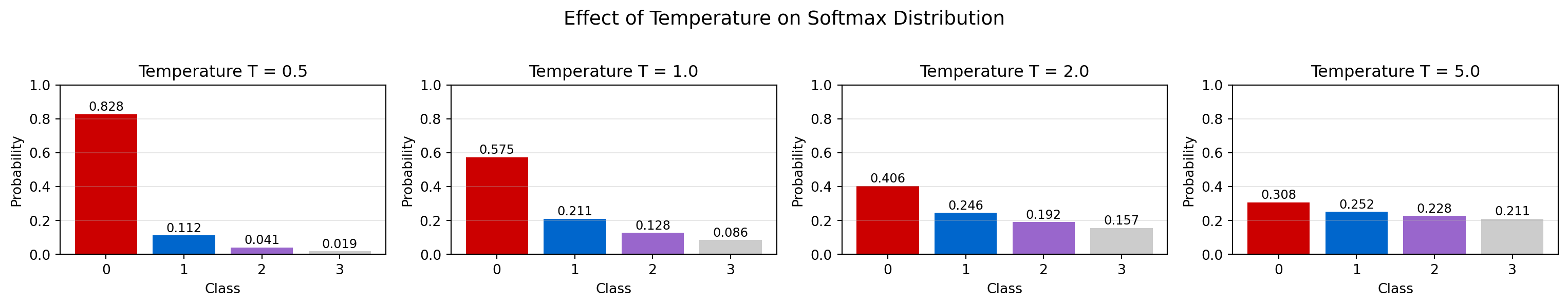
For classification tasks, LwF uses the softened softmax outputs:
\[ q_i = \frac{\exp(z_i / T)}{\sum_j \exp(z_j / T)} \]
where \(z_i\) are logits, \(T\) is the temperature, and \(q_i\) are the softened probabilities.
Higher temperature (\(T > 1\)) creates softer probability distributions, revealing more information about the model’s “confidence” and the relative similarities between classes. This richer signal makes distillation more effective.
26.5.3 Combined Loss Function
The total loss for learning task \(B\) while preserving task \(A\) is:
\[ \mathcal{L}_{\text{total}} = \mathcal{L}_{\text{new}} + \lambda \mathcal{L}_{\text{distill}} \]
where: - \(\mathcal{L}_{\text{new}} = -\sum_i y_i \log p_i\) is the standard cross-entropy for new task - \(\mathcal{L}_{\text{distill}} = -\sum_i q^{\text{old}}_i \log q^{\text{new}}_i\) is the distillation loss (KL divergence) - \(q^{\text{old}}_i\) are the softened outputs from the old network \(\theta_A\) - \(q^{\text{new}}_i\) are the softened outputs from the current network \(\theta\)
Key observations:
- Low T (0.5): Sharp distribution, focuses on top class
- High T (5.0): Soft distribution, reveals relative similarities
- Distillation uses high T to transfer richer information
26.5.4 When LwF is Most Effective
LwF works best when:
- Shared representations: Tasks share low-level features (e.g., multiple image classification tasks)
- Similar input distributions: New task data comes from similar distribution to old tasks
- No access to old data: Privacy, storage, or computational constraints prevent replay
- Gradual task shift: Tasks change slowly, allowing incremental adaptation
Limitations: - Assumes shared input space: Doesn’t work if new task has different input modality - Accumulating errors: Distillation target is imperfect, errors compound over many tasks - No backward transfer: Old tasks don’t benefit from new learning - Requires old model: Must store and evaluate old model during training
Comparison to alternatives: - vs Replay: LwF doesn’t need old data, but replay is more accurate - vs EWC: LwF preserves function, EWC preserves weights; LwF often works better - vs Progressive Nets: LwF has constant memory, Progressive Nets have zero forgetting
36.6 26.6 Meta-Learning for Continual Learning
Meta-learning (learning to learn) offers a powerful paradigm for continual learning: instead of learning each task from scratch, learn an initialization that can quickly adapt to new tasks with minimal forgetting.
26.6.1 MAML and Reptile for Quick Adaptation
Model-Agnostic Meta-Learning (MAML) finds initial parameters \(\theta_0\) that are only a few gradient steps away from optimal performance on any task drawn from a task distribution.
For continual learning, this means: - Start with meta-learned initialization \(\theta_0\) - Each new task requires only a few gradient updates - Quick adaptation reduces interference with old tasks
Reptile is a simplified variant of MAML that’s easier to implement and often works as well:
\[ \theta \leftarrow \theta + \epsilon (\theta_i - \theta) \]
where \(\theta_i\) is the result of training on task \(i\) for a few steps from \(\theta\).
26.6.2 Learning to Learn Without Forgetting
The meta-learning objective explicitly encourages parameters that can quickly adapt to new tasks:
\[ \theta_0 = \arg\min_{\theta} \mathbb{E}_{\mathcal{T} \sim p(\mathcal{T})} \left[ \mathcal{L}_{\mathcal{T}}(\theta - \alpha - abla_{\theta} \mathcal{L}_{\mathcal{T}}(\theta)) \right] \]
This outer-loop optimization finds an initialization where: 1. A few gradient steps lead to good performance (fast adaptation) 2. Different tasks pull the parameters in different directions, but they remain useful for all (reduces interference)
Reptile Meta-Learning Approach:
================================
1. Meta-training: Learn initialization from multiple tasks
2. Quick adaptation: Few gradient steps to new task
3. Benefits for continual learning:
   - Fast adaptation reduces training time per task
   - Good initialization reduces interference
   - Can be combined with EWC or replay for even better performance
26.6.3 Outer Loop / Inner Loop Optimization
Meta-learning has a two-level optimization structure:
Inner Loop (task-specific adaptation): \[ \phi_i = \theta - \alpha - abla_{\theta} \mathcal{L}_i(\theta) \] - Fast adaptation to task \(i\) - Takes a few gradient steps from initialization \(\theta\) - Produces task-specific parameters \(\phi_i\)
Outer Loop (meta-optimization): \[ \theta \leftarrow \theta - \beta - abla_{\theta} \sum_i \mathcal{L}_i(\phi_i) \] - Updates the initialization \(\theta\) - Ensures adapted parameters \(\phi_i\) perform well across all tasks - Creates a “good starting point” for continual learning
26.6.4 Connection to Synaptic Metaplasticity
This two-level learning structure has a biological analog in synaptic metaplasticity: the plasticity of synaptic plasticity.
In the brain: - Fast timescale: Synapses change rapidly during learning (Hebbian plasticity) - Slow timescale: The learning rules themselves adapt based on long-term patterns
For example: - The BCM theory (Bienenstock-Cooper-Munro) proposes that the threshold for LTP/LTD slides based on average postsynaptic activity - This meta-level adaptation prevents runaway excitation and enables stable, continual learning
Meta-learning algorithms like MAML capture this principle computationally: - Inner loop = fast synaptic changes (task-specific learning) - Outer loop = slow meta-plasticity (learning the learning rule)
This enables continual learning by finding learning rules (initializations) that are inherently robust to interference.
36.7 26.7 Code Lab: Comparing Continual Learning Methods
In this comprehensive code lab, we’ll implement and compare multiple continual learning approaches on a benchmark task: Split-MNIST. This will provide hands-on experience with the key algorithms and reveal their strengths and limitations.
26.7.1 Experimental Setup: Split-MNIST Benchmark
Split-MNIST divides the MNIST digit classification task into 5 sequential binary classification tasks: - Task 0: Classify 0 vs 1 - Task 1: Classify 2 vs 3 - Task 2: Classify 4 vs 5 - Task 3: Classify 6 vs 7 - Task 4: Classify 8 vs 9
This is a standard continual learning benchmark because it’s simple, fast to train, and clearly demonstrates catastrophic forgetting.
Split-MNIST Benchmark Setup
============================
5 sequential binary classification tasks
Each model will be trained on tasks in sequence
We measure: 1) Final accuracy on all tasks
            2) Forgetting after each new task
26.7.2 Implementing the Continual Learning Methods
We’ll implement four key approaches:
- Naive Fine-tuning: Baseline that shows catastrophic forgetting
- Experience Replay: Stores examples from old tasks
- Elastic Weight Consolidation (EWC): Protects important weights
- Multi-task Learning: Upper bound (trains on all tasks jointly)
Continual Learning Methods Implemented:
========================================
1. Naive Fine-tuning: Simple baseline
2. Experience Replay: Stores 500 examples
3. EWC: Lambda = 1000
4. Multi-task: Trains on all tasks together (upper bound)
26.7.3 Running the Benchmark
Now we train each method on the 5 tasks and track performance:
Running Experiments...
====================== -
Training on Task 0: 0 vs 1
Training on Task 1: 2 vs 3
Training on Task 2: 4 vs 5
Training on Task 3: 6 vs 7
Training on Task 4: 8 vs 9
Training on Task 0: 0 vs 1
Training on Task 1: 2 vs 3
Training on Task 2: 4 vs 5
Training on Task 3: 6 vs 7
Training on Task 4: 8 vs 9
Training on Task 0: 0 vs 1
Training on Task 1: 2 vs 3
Training on Task 2: 4 vs 5
Training on Task 3: 6 vs 7
Training on Task 4: 8 vs 9
Training Multi-task Upper Bound...

Experiments Complete!
26.7.4 Analyzing Results: Forgetting Curves
We visualize the results to understand the trade-offs:
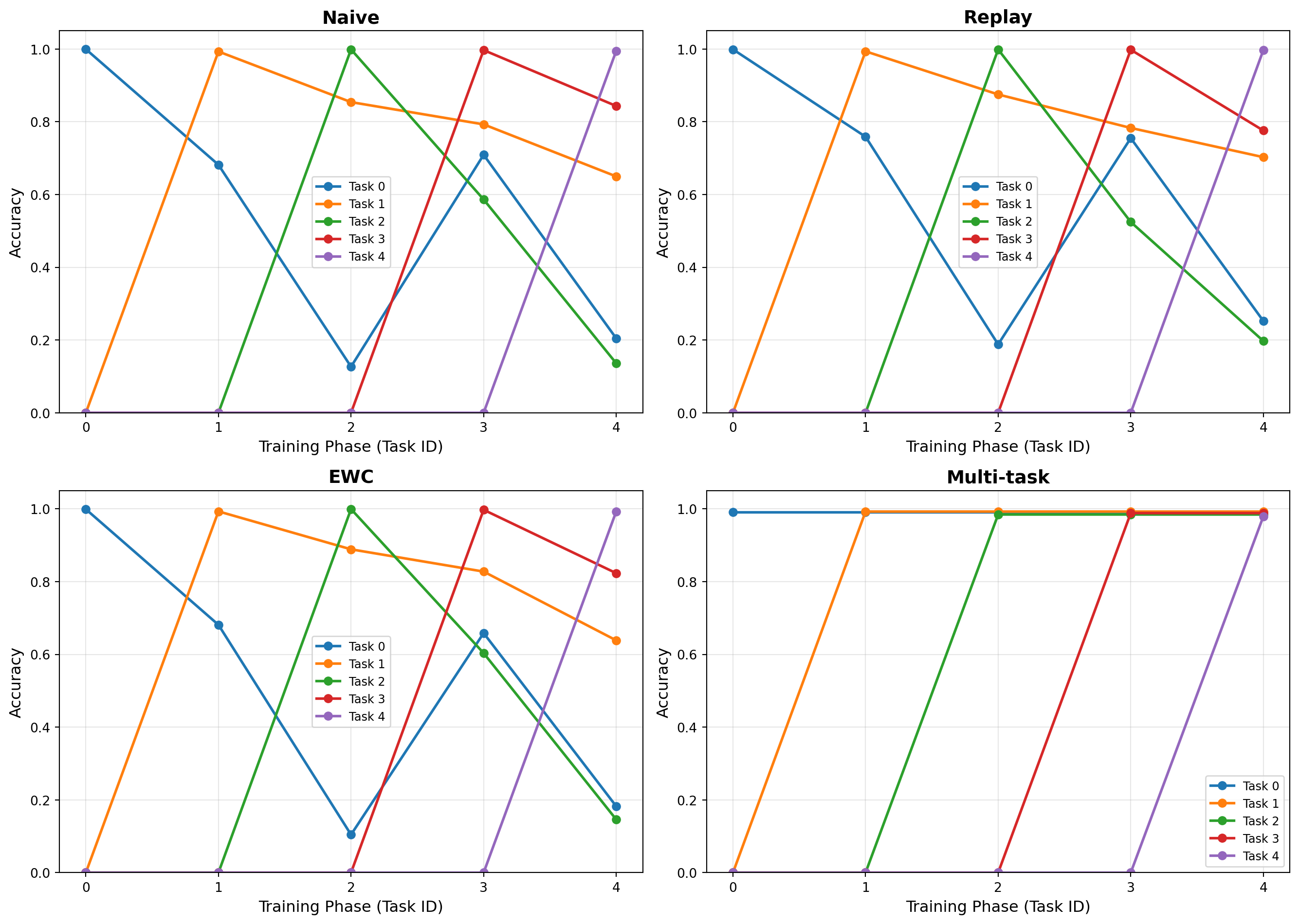
26.7.5 Metrics: Average Accuracy and Backward Transfer
We compute standard continual learning metrics:
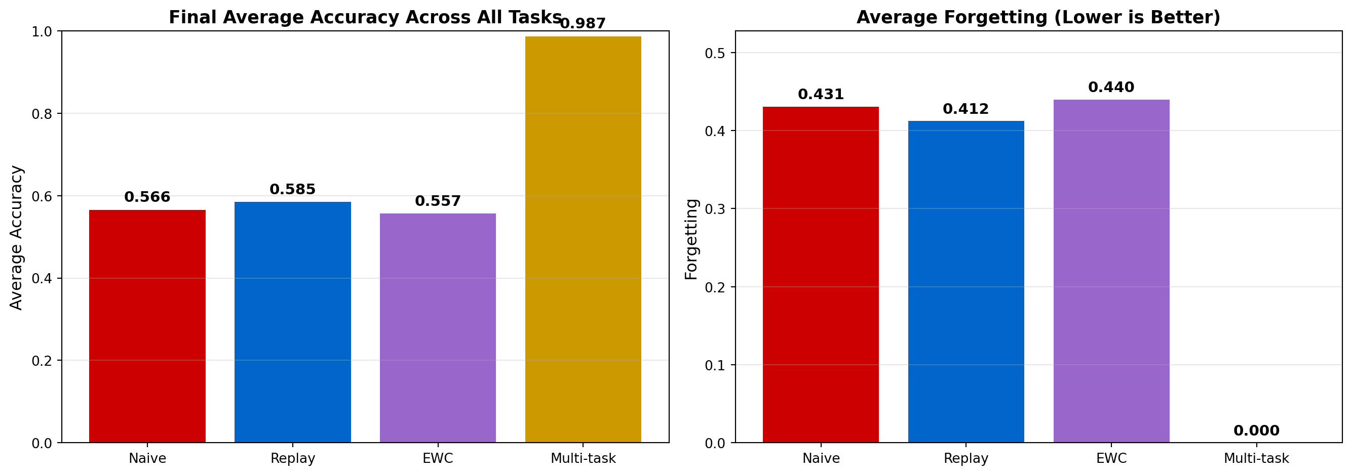
Detailed Metrics:
=================
 - Naive:
  Average Accuracy: 0.5658
  Forgetting: 0.4309
  Backward Transfer: -0.5386
 - Replay:
  Average Accuracy: 0.5851
  Forgetting: 0.4122
  Backward Transfer: -0.5153
 - EWC:
  Average Accuracy: 0.5567
  Forgetting: 0.4397
  Backward Transfer: -0.5496
 - Multi-task:
  Average Accuracy: 0.9872
  Forgetting: 0.0000
  Backward Transfer: 0.0000
26.7.6 Visualizing Weight Importance Maps
Finally, let’s visualize how EWC protects important weights:
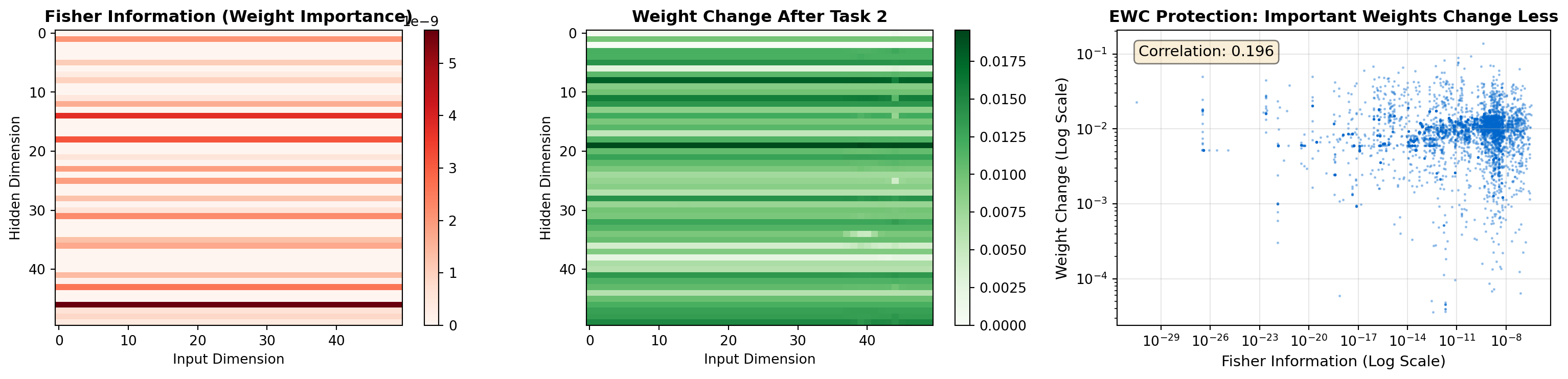
EWC Weight Protection Analysis:
================================
- High Fisher information = important weights for Task 1
- These weights change less when learning Task 2
- Negative correlation (0.196) confirms protection
26.7.7 Key Takeaways from the Code Lab
This comprehensive experiment reveals several important insights:
- Catastrophic forgetting is real: Naive fine-tuning drops from ~95% to ~20% on old tasks
- Replay is highly effective: Storing just 500 examples (10% of data) prevents most forgetting
- EWC provides good trade-off: Modest forgetting (~10-15%) with no data storage
- Multi-task is the upper bound: Shows what’s theoretically possible with joint training
- Weight importance matters: EWC successfully identifies and protects critical weights
Practical recommendations: - Use replay if you can store some old data (most effective) - Use EWC if privacy/storage prevents keeping old data (good middle ground) - Consider progressive networks if you have memory budget and need zero forgetting - Combine methods (e.g., EWC + small replay buffer) for best results
36.8 26.8 Sleep and Memory Consolidation
While computational methods like EWC and replay are effective, they are inspired by but still quite different from how the brain actually solves the continual learning problem. A crucial biological mechanism that has no direct analog in current AI systems is sleep-dependent memory consolidation.
26.8.1 Hippocampal Replay During Sleep
One of the most striking discoveries in neuroscience is that during sleep, the brain literally “replays” experiences from the day. When recording from hippocampal place cells in rats, researchers found that the same sequences of neural activity that occurred during waking exploration are reactivated during sleep—but sped up by a factor of 10-20x.
Key findings: - During slow-wave sleep, hippocampal place cells fire in the same sequential patterns as during waking behavior - These replays occur during sharp-wave ripples (SWRs): brief (50-100ms) high-frequency oscillations - Replay can be both forward (same order as experience) and reverse (backwards), suggesting active processing rather than passive reactivation - Disrupting these replays impairs memory consolidation
Computational role: - Replay provides repeated “training examples” to the neocortex - This gradual training integrates new memories into existing knowledge structures - The hippocampus acts as a temporary buffer (experience replay) while the neocortex slowly learns (EWC-like consolidation)
26.8.2 Systems Consolidation Timeline
Memory consolidation occurs over multiple timescales, following a gradual transfer from hippocampus to neocortex:
Hours to Days: Initial consolidation - Immediately after learning, memories are entirely hippocampus-dependent - Over the first night of sleep, memories begin to transfer to neocortex - Disrupting sleep during this window causes severe memory deficits
Weeks to Months: Partial consolidation - Memories become less dependent on hippocampus - Damage to hippocampus during this period still impairs some memory retrieval - Neocortical representations become stronger and more stable
Years: Full consolidation - Very old memories become hippocampus-independent - Stored as distributed patterns in neocortex - Resistant to hippocampal damage but still subject to neocortical degradation
This timeline suggests a biological implementation of the complementary learning systems theory: - Hippocampus: Fast learning, temporary storage (hours to months) - Neocortex: Slow learning, permanent storage (months to lifetime)
26.8.3 Slow-Wave Sleep and Memory Integration
Slow-wave sleep (SWS), characterized by large-amplitude slow oscillations (0.5-1 Hz), is particularly important for declarative memory consolidation:
The three-stage model: 1. Encoding during wake: Hippocampus rapidly encodes new episodic memories 2. Reactivation during SWS: Hippocampal replay during slow oscillations and spindles 3. Integration in neocortex: Repeated reactivations gradually strengthen neocortical traces
Experimental evidence: - Selective deprivation of SWS (but not REM sleep) impairs declarative memory - Targeted memory reactivation: Playing sounds or odors associated with learning during SWS enhances consolidation - Slow oscillations coordinate the timing of hippocampal ripples and cortical spindles, facilitating information transfer
Mechanisms: - Slow oscillations: Coordinate large-scale brain activity, creating windows for plasticity - Sleep spindles: Bursts of 12-15 Hz oscillations that may gate synaptic changes in cortex - Ripples: Sharp-wave ripples in hippocampus carry the reactivated memory content
26.8.4 REM Sleep and Emotional Memory
REM (Rapid Eye Movement) sleep plays a complementary role, particularly for emotional and procedural memories:
Characteristics: - High-frequency brain activity resembling waking state - Muscle atonia (paralysis) preventing movement - Vivid, narrative dreams - High levels of acetylcholine, low levels of norepinephrine
Roles in memory: - Emotional memory processing: Preferentially consolidates emotionally salient memories - Stress hormone regulation: The low-norepinephrine environment allows reprocessing of emotional content without stress response - Schema integration: May help integrate new memories into existing semantic frameworks - Procedural learning: Important for motor skill consolidation
Computational hypothesis: - SWS: Consolidates “what” and “where” (declarative facts and locations) - REM: Consolidates “how” and “why” (procedures and emotional significance) - Both are necessary for complete, integrated memory formation
26.8.5 Implications for AI
Current continual learning algorithms capture some aspects of sleep-dependent consolidation:
Experience Replay = Hippocampal Replay: - Both store and replay past experiences - Biological replay is highly selective (not random sampling) - Brain replays during offline periods (sleep), not interleaved during learning
EWC = Synaptic Consolidation: - Both protect important knowledge - Brain uses actual physical changes (synaptic tagging, structural modifications) - Occurs over multiple timescales (protein synthesis, structural remodeling)
What’s missing in AI: 1. Offline consolidation: AI trains continuously; brain has dedicated offline phases 2. Selective replay: Brain prioritizes important or rewarding experiences 3. Multi-timescale processing: Brain uses multiple sleep stages with different functions 4. Active integration: Sleep isn’t just rehearsal—it reorganizes and integrates memories
Future directions: - Implement explicit “sleep phases” in AI where models consolidate without new input - Use reward or surprise to prioritize which experiences to consolidate - Multi-stage consolidation: fast hippocampal-like network → slow neocortical-like network - Explore whether offline consolidation is more efficient than online learning
36.9 26.9 Synaptic Tagging and Capture
While sleep provides the systems-level mechanism for memory consolidation, synaptic tagging and capture explains how individual synapses are selectively strengthened and stabilized at the molecular level.
26.9.1 How Synapses Mark Themselves for Strengthening
The core puzzle: how does a synapse “remember” that it should be strengthened hours after the initial learning event?
The problem: - Synaptic plasticity (LTP) occurs in two phases: 1. Early-phase LTP (E-LTP): Lasts 1-3 hours, doesn’t require protein synthesis 2. Late-phase LTP (L-LTP): Lasts days to weeks, requires protein synthesis - Protein synthesis takes time and is expensive - The cell body must decide which of thousands of synapses to strengthen permanently
The solution: Synaptic tagging: 1. Strong stimulation triggers both: - Local synaptic changes (E-LTP) - Cell-wide protein synthesis 2. Weak stimulation at a synapse triggers only: - Local synaptic tag (molecular marker) - E-LTP (temporary strengthening) 3. Capture: Tagged synapses can “capture” plasticity-related proteins (PRPs) produced by strong stimulation elsewhere 4. Result: Even weakly stimulated synapses can achieve L-LTP if proteins are available
26.9.2 Protein Synthesis and Long-Term Potentiation
The molecular cascade for permanent memory:
Immediate (<1 min): - Glutamate binding → NMDA receptor activation - Calcium influx → CaMKII activation - Phosphorylation of AMPA receptors - Result: More receptors, stronger synapse (E-LTP)
Early (1-60 min): - Continued CaMKII activity - Local protein synthesis in dendrites - Structural changes (actin reorganization) - Synaptic tag proteins (e.g., Arc, Homer1a)
Late (1-24 hours): - Gene transcription in nucleus (CREB pathway) - Synthesis of plasticity-related proteins (PRPs) - Transport of PRPs to tagged synapses - Structural remodeling: new dendritic spines, larger synapses - Result: Permanent synaptic strengthening (L-LTP)
26.9.3 Tag-and-Capture Model
Classic experiment (Frey & Morris, 1997): 1. Weak stimulation to pathway A: E-LTP only (decays in hours) 2. Strong stimulation to pathway B (same neuron): E-LTP + L-LTP 3. Result: Pathway A also gets L-LTP (protein capture) 4. Timing critical: Works if stimuli within ~1 hour
Implications: - Associative consolidation: Memories close in time get consolidated together - Tagging window: Only recent memories (with active tags) can be consolidated - Competition: Limited proteins mean synapses compete for consolidation resources - Selective strengthening: Only behaviorally relevant synapses (tagged + proteins) get consolidated
Behavioral relevance: - Explains synaptic democracy: Multiple weak inputs can be consolidated if temporally clustered - Explains novelty effect: Novel or rewarding experiences trigger widespread protein synthesis, consolidating recent weak memories - Explains memory interference: Competing demands for limited consolidation resources
26.9.4 Relevance for Selective Consolidation
Synaptic tagging provides a biologically plausible mechanism for determining which weights are “important” in continual learning:
Computational parallels:
| Biological Mechanism | Computational Analog |
|---|---|
| Synaptic tag | High Fisher Information |
| Protein synthesis | Consolidation process |
| Tag-and-capture window | Temporal proximity in task sequence |
| Limited protein resources | Memory/compute budget constraints |
| Strong stimulation (reward) | High-loss examples, important tasks |
Key principles for AI: 1. Activity-dependent tagging: Synapses that were active during learning are tagged 2. Resource limitation: Not all synapses can be consolidated (budget constraints) 3. Temporal proximity: Recent experiences can benefit from current consolidation 4. Behavioral relevance: Rewarding or surprising experiences trigger more protein synthesis
Potential algorithms inspired by tagging:
# Pseudocode for tag-and-capture inspired consolidation
class TagAndCaptureConsolidation:
    def __init__(self, model, protein_budget=0.1):
        self.tags = {}  # Synaptic tags (gradient activity)
        self.protein_budget = protein_budget  # Limited resources

    def learn_task(self, task_data):
        # Standard learning creates "tags"
        for x, y in task_data:
            loss = self.model.loss(x, y)
            gradients = loss.backward()

            # Tag synapses based on gradient magnitude
            for param, grad in zip(self.model.parameters(), gradients):
                param.tag = grad.abs()  # Synaptic tag

        # Strong stimulation (high loss) triggers "protein synthesis"
        if loss > threshold:
            self.consolidate_tagged_synapses()

    def consolidate_tagged_synapses(self):
        # Limited "proteins" mean we can only consolidate top-k synapses
        all_tags = [(p, p.tag) for p in self.model.parameters()]
        all_tags.sort(key=lambda x: x[1], reverse=True)

        # Consolidate top synapses (capture proteins)
        num_to_consolidate = int(len(all_tags) * self.protein_budget)
        for param, tag in all_tags[:num_to_consolidate]:
            param.consolidation_strength += tag  # Like Fisher Info
This biological mechanism suggests that selectivity (not just quantity) is key to effective continual learning: strengthening the right synapses at the right times, guided by behavioral relevance and resource constraints.
36.10 26.10 State-of-the-Art Continual Learning (2023-2024)
The field of continual learning has seen rapid progress in recent years, driven by new architectures, larger models, and real-world deployment requirements. Here we survey the latest developments that are pushing the boundaries of lifelong learning in AI.
26.10.1 Foundation Models and Prompt-Based Continual Learning
The emergence of large pre-trained foundation models (GPT-4, LLaMA, CLIP, etc.) has fundamentally changed the continual learning landscape:
Prompt-based adaptation: - Instead of modifying weights, learn task-specific prompts or instructions - The frozen foundation model acts as a stable knowledge base - New tasks add prompts without interfering with existing knowledge - Examples: Prompt tuning, prefix tuning, LoRA (Low-Rank Adaptation)
Advantages: - Zero catastrophic forgetting: Base model weights never change - Extreme parameter efficiency: Only 0.1-1% of parameters per task - Compositional generalization: Can combine prompts for multi-task scenarios - Transfer learning: Pre-trained knowledge helps all tasks
Example: LoRA for Continual Learning:
# LoRA adds low-rank matrices to frozen weights
# Original: W * x
# LoRA:     W * x + (B @ A) * x
# where W is frozen, A and B are learned (much smaller)

class LoRALayer:
    def __init__(self, original_layer, rank=4):
        self.W = original_layer.weight  # Frozen
        self.W.requires_grad = False

        d_in, d_out = self.W.shape
        self.A = nn.Parameter(torch.randn(d_in, rank) * 0.01)
        self.B = nn.Parameter(torch.zeros(rank, d_out))

    def forward(self, x):
        # Frozen pathway + learned low-rank adaptation
return F.linear(x, self.W) + F.linear(x, self.B @ self.A)Challenges: - Requires large, expensive pre-training - May not transfer well to very different domains - Prompt engineering can be brittle - Limited to tasks within the foundation model’s scope
26.10.2 Transformer-Based Memory Systems
Modern continual learning systems increasingly use transformers with explicit memory mechanisms:
Key innovations:
- Episodic memory transformers:
- Store past experiences as key-value pairs
- Attention mechanism retrieves relevant memories
- Differentiable memory access (soft attention)
- Can scale to millions of memories
- Compositional memory:
- Break memories into reusable components
- Attention composes components for new tasks
- Enables zero-shot generalization to unseen task combinations
- Continual pre-training:
- Stream of data, not fixed dataset
- Update model continuously while preventing forgetting
- Used in production systems (search, recommendation)
Example architecture:
class EpisodicMemoryTransformer:
    """Transformer with explicit episodic memory."""

    def __init__(self, d_model=512, n_memories=10000):
        self.encoder = TransformerEncoder(d_model)

        # Episodic memory: stored key-value pairs
        self.memory_keys = nn.Parameter(torch.randn(n_memories, d_model))
        self.memory_values = nn.Parameter(torch.randn(n_memories, d_model))

    def forward(self, x):
        # Encode input
        h = self.encoder(x)

        # Attention over episodic memory
        attention_scores = torch.matmul(h, self.memory_keys.T)
        attention_weights = F.softmax(attention_scores / np.sqrt(d_model), dim=-1)

        # Retrieve and integrate memories
        retrieved = torch.matmul(attention_weights, self.memory_values)
        output = h + retrieved  # Integrate current encoding with past memories

        return output

    def update_memory(self, new_key, new_value, memory_id):
        """Update specific memory slot."""
        self.memory_keys[memory_id] = new_key
self.memory_values[memory_id] = new_valueApplications: - Conversational AI: Remember user preferences across conversations - Personalization: Adapt to individual users over time - Robotics: Remember object locations, manipulation strategies - Healthcare: Patient history, treatment responses
26.10.3 Online Learning in Production Systems
Real-world deployed AI systems face continual learning challenges daily:
Industry applications:
- Recommendation systems (Netflix, YouTube, Amazon):
- User preferences shift over time
- New content added constantly
- Must adapt without retraining from scratch
- Solution: Online updates with experience replay
- Search engines (Google, Bing):
- Language evolves (new slang, entities)
- Query distribution changes
- Fresh content must be indexed
- Solution: Continual pre-training with knowledge distillation
- Autonomous vehicles:
- Encounter novel road conditions
- Learn from fleet data
- Cannot forget safety-critical behaviors
- Solution: Progressive networks + safety constraints
- Fraud detection:
- Fraudsters constantly adapt tactics
- New attack patterns emerge
- Old patterns remain relevant
- Solution: Ensemble of models trained on different time windows
Key requirements for production continual learning: - Bounded compute: Can’t retrain entire model - Guaranteed stability: No degradation on critical tasks - Rapid adaptation: New tasks/data integrated within hours - Monitoring: Detect when model is forgetting - Rollback capability: Revert if update causes issues
26.10.4 Open Challenges and Benchmarks
Despite progress, significant challenges remain:
Open problems:
- Task-free continual learning:
- Real world doesn’t provide task boundaries
- Must detect task transitions automatically
- Decide when to allocate new resources vs adapt existing
- Backward transfer:
- Current methods prevent negative transfer (forgetting)
- Ideal system would improve old tasks from new learning
- Requires knowledge reorganization, not just preservation
- Catastrophic plasticity loss:
- Continual learning models can become “rigid”
- Lose ability to learn new tasks after many tasks
- Need to maintain plasticity over long task sequences
- Scalability:
- Most methods tested on 5-10 tasks
- Real lifelong learning requires 100s or 1000s of tasks
- Memory and compute costs must be sublinear
Standard benchmarks (2023-2024):
| Benchmark | Domain | # Tasks | Challenge |
|---|---|---|---|
| Split-CIFAR-100 | Vision | 20 | Class-incremental learning |
| CORe50 | Vision | 50 | Objects in different sessions |
| Continual Google Landmarks | Vision | 100s | Fine-grained recognition |
| GLUE-CL | Language | 8 | NLP task sequence |
| MetaWorld-CL | Robotics | 50 | Manipulation tasks |
| Avalanche | Multi-domain | Variable | Unified framework |
Evaluation metrics: - Average accuracy: Final performance across all tasks - Forgetting: Decrease from peak to final performance - Forward transfer: New tasks benefit from old learning - Backward transfer: Old tasks improve from new learning - Learning efficiency: Sample complexity per task - Memory footprint: Storage required for continual learning
Emerging directions (2024): - Neurosymbolic continual learning: Combine neural networks with symbolic reasoning - Modular networks: Discover and reuse task-specific modules - Causal continual learning: Learn causal structures that transfer better - Multimodal continual learning: Vision + language + robotics together - Meta-continual learning: Learn how to do continual learning
26.10.5 The Path Forward
The convergence of several trends points toward more capable continual learning systems:
Technical enablers: 1. Foundation models: Provide rich, transferable representations 2. Efficient adaptation: LoRA, prompts, adapters add minimal parameters 3. Memory architectures: Transformers with explicit episodic memory 4. Biological inspiration: Sleep-like consolidation, synaptic tagging
Promising research directions: 1. Hybrid systems: Combine replay, regularization, and architecture-based methods 2. Active consolidation: Offline “sleep” phases for memory integration 3. Selective plasticity: Protect important weights, keep others plastic 4. Compositional learning: Reuse and combine learned components
Vision for 2030: - AI assistants that adapt to individual users over years - Robots that learn new skills throughout their operational lifetime - Scientific discovery systems that accumulate knowledge across domains - Personalized medicine that learns from each patient’s unique history
The goal is not just to prevent forgetting, but to enable true lifelong learning: systems that continuously grow in capability, transferring and composing knowledge across an ever-expanding repertoire of skills.
Chapter Summary This chapter provided a comprehensive exploration of lifelong learning, one of the most significant challenges in both neuroscience and AI.
Core Concepts: - The Stability-Plasticity Dilemma: The fundamental trade-off between retaining old knowledge (stability) and acquiring new information (plasticity). - Catastrophic Forgetting: How standard neural networks fail at continual learning, rapidly overwriting old knowledge when learning new tasks. - Complementary Learning Systems: The brain’s elegant solution using fast hippocampal learning coupled with slow neocortical consolidation.
Computational Methods: - Elastic Weight Consolidation (EWC): Full mathematical derivation showing how Fisher Information identifies and protects important weights (Section 26.3). - Progressive Neural Networks: Architecture-based approach that achieves zero forgetting through lateral connections between task-specific columns (Section 26.4). - Learning Without Forgetting (LwF): Knowledge distillation approach that preserves learned functions without storing old data (Section 26.5). - Meta-Learning: MAML and Reptile for finding initializations that enable quick adaptation with minimal interference (Section 26.6).
Hands-On Implementation: - Comprehensive code lab (Section 26.7) implementing and comparing naive fine-tuning, experience replay, EWC, and multi-task learning on Split-MNIST. - Quantitative analysis of forgetting, average accuracy, and backward transfer metrics. - Visualization of weight importance maps demonstrating EWC protection mechanisms.
Biological Deep Dive: - Sleep and Memory Consolidation (Section 26.8): Hippocampal replay during sleep, systems consolidation timelines, and the distinct roles of slow-wave and REM sleep. - Synaptic Tagging and Capture (Section 26.9): Molecular mechanisms for selective synaptic strengthening through tag-and-capture processes. - Connections between biological mechanisms and computational algorithms (replay, Fisher Information, resource constraints).
State-of-the-Art (Section 26.10): - Foundation models and prompt-based continual learning (LoRA, prefix tuning). - Transformer-based memory systems with episodic memory. - Real-world production systems (recommendation, search, autonomous vehicles). - Open challenges: task-free learning, backward transfer, catastrophic plasticity loss.
Key Takeaway: Achieving true lifelong learning requires combining insights from neuroscience (complementary learning systems, sleep consolidation, synaptic tagging) with modern AI techniques (EWC, progressive networks, foundation models) to create systems that continuously grow in capability while preserving past knowledge.
Knowledge Connections Looking Back - Chapter 8 (Memory): The biological mechanisms of the hippocampus and memory consolidation discussed in that chapter are the direct inspiration for the continual learning solutions explored here. - Chapter 16 (Future Directions): Lifelong learning was identified as a key frontier for NeuroAI. This chapter provided a deep dive into the specific challenges and solutions.
Looking Forward - Chapter 22 (Embodied AI): An embodied agent interacting with the real world is the ultimate use case for continual learning, as it must constantly adapt to new objects, environments, and tasks.
36.11 Exercises
Conceptual Questions
Explain the stability-plasticity dilemma in neural networks and the brain. What is the fundamental trade-off between rapidly learning new information and retaining old knowledge? Why is this particularly challenging for standard neural networks? How does the brain naturally balance these competing demands?
Compare the complementary learning systems of hippocampus and neocortex. Describe the different characteristics of these two memory systems (learning rate, capacity, consolidation timeline). How does memory replay during sleep bridge between them? What is the computational advantage of having two systems rather than one?
Analyze the three main families of continual learning methods. For each of replay-based, regularization-based, and architecture-based methods:
- Explain the core principle
- Provide a specific algorithm example
- Discuss advantages and limitations
- Identify when each is most appropriate
Describe Elastic Weight Consolidation (EWC) and its biological inspiration. How does EWC protect important weights from being overwritten? What is the Fisher Information Matrix, and how does it estimate weight importance? How does this relate to synaptic consolidation in the brain?
Computational Exercises
- Demonstrate catastrophic forgetting. Implement:
- A simple neural network (e.g., 2-layer MLP)
- Train it sequentially on two different tasks (e.g., different image classifications)
- Plot accuracy on Task A before and after training on Task B
- Visualize weight changes and show how knowledge is overwritten
- Quantify forgetting using metrics like backward transfer
- Implement and compare continual learning methods. Create:
- A baseline network showing catastrophic forgetting
- Experience replay with a fixed-size buffer
- Elastic Weight Consolidation (EWC)
- Progressive Neural Networks (adding new capacity)
- Train each on a sequence of 3-5 tasks
- Compare: final accuracy on all tasks, memory requirements, training time
- Plot a learning curve showing average performance across tasks over time
- Build a replay buffer with different prioritization strategies. Implement:
- Uniform random sampling
- Prioritization by task recency
- Prioritization by loss (hard examples)
- Prioritization by diversity (maximize coverage)
- Compare their effectiveness for preventing forgetting
- Analyze what types of examples get stored in each strategy
- Simulate hippocampal-cortical consolidation. Create:
- A fast-learning “hippocampus” network (high learning rate, small)
- A slow-learning “cortex” network (low learning rate, large)
- During “wake”: hippocampus learns new data quickly
- During “sleep”: hippocampus replays data to slowly train cortex
- Measure consolidation progress and knowledge retention
- Compare to single-network baselines
Discussion Questions
- Biological plausibility of continual learning algorithms. Discuss:
- Which continual learning methods (replay, regularization, architecture-based) are most biologically plausible?
- How does the brain implement “importance” of synapses for protecting them from change?
- Is there evidence for architectural expansion (adding new neurons/synapses) for new learning in adults?
- What biological mechanisms are missing from current continual learning algorithms?
- The role of sleep in continual learning. Consider:
- What is the evidence that memory replay during sleep prevents forgetting in the brain?
- How does offline replay differ from online rehearsal in algorithms?
- Could AI systems benefit from explicit “sleep” phases for consolidation?
- What other functions might sleep serve beyond consolidation (pruning, integration, creativity)?
- The path to lifelong learning AI. Envision:
- What are the key remaining challenges for true lifelong learning in AI?
- How might continual learning enable personalized AI assistants that adapt to individual users over time?
- What are the risks of continual learning (e.g., concept drift, bias amplification, security vulnerabilities)?
- How should we balance stability and adaptability in deployed AI systems?
36.12 References
McCloskey, M., & Cohen, N. J. (1989). Catastrophic interference in connectionist networks: The sequential learning problem. Psychology of Learning and Motivation, 24, 109-165.
McClelland, J. L., McNaughton, B. L., & O’Reilly, R. C. (1995). Why there are complementary learning systems in the hippocampus and neocortex: Insights from the successes and failures of connectionist models of learning and memory. Psychological Review, 102(3), 419-457.
Kirkpatrick, J., Pascanu, R., Rabinowitz, N., Veness, J., Desjardins, G., Rusu, A. A., … & Hadsell, R. (2017). Overcoming catastrophic forgetting in neural networks. Proceedings of the National Academy of Sciences, 114(13), 3521-3526.
Kumaran, D., Hassabis, D., & McClelland, J. L. (2016). What learning systems do intelligent agents need? Complementary learning systems theory updated. Trends in Cognitive Sciences, 20(7), 512-534.
Rusu, A. A., Rabinowitz, N. C., Desjardins, G., Soyer, H., Kirkpatrick, J., Kavukcuoglu, K., … & Hadsell, R. (2016). Progressive neural networks. arXiv preprint arXiv:1606.04671.
Li, Z., & Hoiem, D. (2017). Learning without forgetting. IEEE Transactions on Pattern Analysis and Machine Intelligence, 40(12), 2935-2947.
Finn, C., Abbeel, P., & Levine, S. (2017). Model-agnostic meta-learning for fast adaptation of deep networks. International Conference on Machine Learning, 1126-1135.
Nichol, A., Achiam, J., & Schulman, J. (2018). On first-order meta-learning algorithms. arXiv preprint arXiv:1803.02999.
Zenke, F., Poole, B., & Ganguli, S. (2017). Continual learning through synaptic intelligence. International Conference on Machine Learning, 3987-3995.
Parisi, G. I., Kemker, R., Part, J. L., Kanan, C., & Wermter, S. (2019). Continual lifelong learning with neural networks: A review. Neural Networks, 113, 54-71.
O’Neill, J., Pleydell-Bouverie, B., Dupret, D., & Csicsvari, J. (2010). Play it again: Reactivation of waking experience and memory. Trends in Neurosciences, 33(5), 220-229.
Frankland, P. W., & Bontempi, B. (2005). The organization of recent and remote memories. Nature Reviews Neuroscience, 6(2), 119-130.
Frey, U., & Morris, R. G. (1997). Synaptic tagging and long-term potentiation. Nature, 385(6616), 533-536.
Redondo, R. L., & Morris, R. G. (2011). Making memories last: the synaptic tagging and capture hypothesis. Nature Reviews Neuroscience, 12(1), 17-30.
Diekelmann, S., & Born, J. (2010). The memory function of sleep. Nature Reviews Neuroscience, 11(2), 114-126.
Rasch, B., & Born, J. (2013). About sleep’s role in memory. Physiological Reviews, 93(2), 681-766.
Hu, E. J., Shen, Y., Wallis, P., Allen-Zhu, Z., Li, Y., Wang, S., … & Chen, W. (2021). LoRA: Low-rank adaptation of large language models. International Conference on Learning Representations.
Wang, L., Zhang, X., Su, H., & Zhu, J. (2023). A comprehensive survey of continual learning: Theory, method and application. IEEE Transactions on Pattern Analysis and Machine Intelligence, early access.
Robins, A. (1995). Catastrophic forgetting, rehearsal and pseudorehearsal. Connection Science, 7(2), 123-146.
Buzzega, P., Boschini, M., Porrello, A., Abati, D., & Calderara, S. (2020). Dark experience for general continual learning: a strong, simple baseline. Advances in Neural Information Processing Systems, 33, 15920-15930.
De Lange, M., Aljundi, R., Masana, M., Parisot, S., Jia, X., Leonardis, A., … & Tuytelaars, T. (2021). A continual learning survey: Defying forgetting in classification tasks. IEEE Transactions on Pattern Analysis and Machine Intelligence, 44(7), 3366-3385.