6 A Long-Standing Dialogue: Neuroscience and AI
6.1 Learning Objectives
By the end of this chapter, you will be able to:
- Understand the historical dialogue between neuroscience and AI as two fields asking the same fundamental questions.
- Appreciate the artificial neuron as a “brilliant caricature” of its biological counterpart.
- Trace the co-evolution of the fields through three major acts: an initial spark, a period of divergence, and a grand re-convergence.
- Explain how key neuroscientific principles like hierarchical processing and reward prediction have inspired major AI advances.
- Recognize that AI now serves as a powerful tool for advancing neuroscience research, completing a virtuous cycle.
6.2 1.1 The Core Question and the Two Fields
How does intelligence work? For over a century, two fields have pursued this question from different directions.
- Neuroscience starts with the hardware—the wet, complex, and messy biological brain—and works to deduce the principles of its operation.
- Artificial Intelligence starts with the principles—logic, mathematics, and computation—and works to build intelligent hardware and software from scratch.
This handbook is about the rich, decades-long dialogue between them. It’s a story of a conversation, where each field has taken turns inspiring, challenging, and profoundly advancing the other. Across the past eight decades, this dialogue has moved through three acts: an initial spark, a divergence, and a powerful re-convergence.
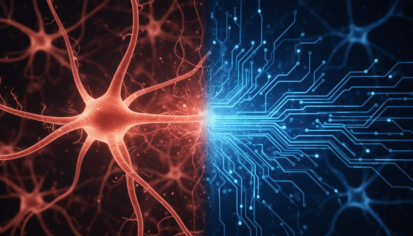
At the heart of this dialogue is a single, powerful idea: the artificial neuron as a brilliant caricature of the biological neuron. It is a deliberate simplification that discards many messy biological details while capturing a core computational essence: integrate inputs, apply a transformation, emit an output. While no single artificial neuron captures the full richness of cellular physiology, the abstraction has proven sufficient to build powerful systems and to formulate and test theories about intelligence.

Figure 1.1: The central analogy. The artificial neuron is a simplified model—a caricature—of the biological neuron, capturing core computational function while abstracting away metabolic and cellular detail. Left: biological neuron. Right: artificial perceptron.
Warning: The artificial neuron is a caricature, not a miniaturised copy, of a cortical column.
- Simplification aids engineering, but resemblance alone does not imply mechanistic equivalence.
- Architectural depth (e.g., deep ReLU stacks) is not evidence of cortical homology.
- Claims of “just like the brain” must specify which of Marr’s levels align—algorithmic similarity is possible without implementational likeness.
- Guardrails: respect the analogy, resist the mirage.
6.3 1.2 Act I: The Spark of Inspiration (1940s–1960s)
The earliest days of computing and AI were inseparable from the quest to understand the brain. The pioneers of AI were not only computer scientists; they were trying to reverse-engineer the mind.
Thinking as Computation
A first revolutionary insight was that thinking could be described as a form of computation. In 1943, Warren McCulloch and Walter Pitts proposed a mathematical model of a neuron: a binary threshold unit that fires if a weighted sum of inputs exceeds a threshold. They showed that networks of such units can, in principle, compute any logical function via Boolean circuits (McCulloch & Pitts 1943). This was a profound philosophical leap: the mysterious processes of the mind could be grounded in formal logic and mathematics.
Key ideas: - Binary threshold units as formal neurons - Composition of simple units to realise complex logic - Early bridge between neurobiology and computation
Learning by Correcting Errors
The next leap was to make these networks learn from data. In 1957–1958, Frank Rosenblatt introduced the Perceptron, a linear classifier trained with an error-correction learning rule that adjusts weights to reduce mistakes (Rosenblatt 1958). Unlike the fixed McCulloch–Pitts units, perceptrons used data-driven learning to improve performance on classification tasks.
The Perceptron delivered proof-of-concept demonstrations of machine learning and showcased how simple, brain-inspired rules could yield adaptive behaviour.
Cross-Currents: Cybernetics and Control Theory
Before the perceptron, cybernetics provided a shared vocabulary that kept engineers and neuro-physiologists “in the same room.”
- Norbert Wiener’s Cybernetics (1948) cast the brain and automatic machines as feedback controllers, normalising talk of goals, error signals, and negative feedback.
- W. Ross Ashby’s Design for a Brain (1952) formalised homeostasis and adaptation, persuading biologists that control-theoretic abstractions could illuminate neural function.
Least-mentioned but highly influential sources include: - Jerome Lettvin’s “What the Frog’s Eye Tells the Frog’s Brain” (1959), a proof-of-concept for feature-specific neurons predating Hubel & Wiesel. - Rosenblatt <-> Selfridge (1959). Heated exchanges over perceptron learning versus Oliver Selfridge’s “Pandemonium” demons foreshadowed today’s error-backprop vs. symbolic rule-induction debates.
6.4 1.3 Act II: The Great Divergence (1970s–1980s)
The early excitement soon met hard limits. In 1969, Marvin Minsky and Seymour Papert’s book Perceptrons rigorously analysed single-layer perceptrons and showed they cannot represent certain non-linearly separable functions (e.g., XOR) under standard encodings (Minsky & Papert 1969). Although multi-layer networks were known, efficiently training them remained a bottleneck. Combined with limited compute and data, this contributed to the first AI winter.
During this period, the two fields drifted: - AI largely shifted to symbolic AI, emphasising logic, rules, and expert systems. This approach excelled at explicit reasoning but struggled with perception, robustness, and learning from raw data. - Neuroscience, empowered by new experimental techniques and a surge in molecular and systems biology, dove deeper into biological mechanisms—ion channels, neurotransmitters, synaptic plasticity—moving away from the simple abstractions that had energised early AI.
The dialogue quieted. The fields continued asking similar questions about representation, learning, and computation, but they no longer spoke the same language.
6.5 1.4 Act III: The Grand Re-Convergence (1980s–Present)
The conversation reignited in the 1980s with the popularisation of the backpropagation algorithm (Rumelhart, Hinton & Williams 1986), building on earlier ideas (Werbos 1974). Backpropagation provided an efficient way to compute gradients layer by layer, enabling practical training of multi-layer neural networks and overcoming the core limitation identified by Minsky and Papert. This reopened the door to learning complex, nonlinear functions from data.
The deep learning wave of the 2010s amplified this shift. Massive datasets, GPU parallelism, and architectural innovations produced striking advances across perception, language, and decision-making. Notable milestones include ImageNet breakthroughs (Krizhevsky, Sutskever & Hinton 2012), superhuman gameplay (AlphaGo; Silver et al. 2016), and large language models (2018–2023). These successes brought neuroscience and AI back into close alignment, catalysing a modern, virtuous cycle.
The Virtuous Cycle of NeuroAI
Today, the dialogue is more vibrant than ever: - Neuroscience inspires AI. The hierarchical organisation of the visual cortex (Hubel & Wiesel 1962) and the Neocognitron (Fukushima 1980) directly informed modern Convolutional Neural Networks (LeCun et al. 1989, 1998). Similarly, the brain’s reward-prediction mechanisms—dopaminergic prediction-error signals—align with Temporal-Difference (TD) learning (Sutton 1988) and underpin modern Reinforcement Learning (Sutton & Barto 2018). - AI advances neuroscience. Deep learning and probabilistic modelling now help decode neural population activity, reconstruct connectomes, and serve as candidate models of cortical computation. As we will see in later chapters, AI models are increasingly used as testable theories of brain function, linking stimuli, neural responses, and behaviour.
6.6 1.5 Core Principles and Mathematical Glimpses
To bridge intuition with formalism, here are brief mathematical touchpoints that connect biological and artificial perspectives. These are teasers; later chapters expand each in depth.
Biological Neurons: Leaky Integrate-and-Fire (LIF)
A simplified dynamical model of membrane potential V(t) with time constant τm:
\[\tau_m \frac{dV}{dt} = -(V - V_{rest}) + R_m I(t)\]
- \(\tau_m\): membrane time constant
- \(V_{rest}\): resting potential
- \(R_m\): membrane resistance
- \(I(t)\): synaptic/input current
A spike is emitted when V crosses a threshold, after which V resets to \(V_{rest}\).
Artificial Neurons: Linear + Non-Linearity
A minimal artificial neuron computes \(y = \phi(w \cdot x + b)\). For ReLU:
\[y = \max(0, w^T x + b)\]
Population Dynamics (Rate Models)
At the mesoscopic level, population activity r(t) can be modelled as:
\[\frac{dr}{dt} = -r + f(W r + I_{ext})\]
where W is connectivity and f is a nonlinear activation function. These abstractions connect circuit structure to emergent computations.
Plasticity Glimpse: BCM Rule
A stylised synaptic-plasticity rule:
\[\Delta w_{ij} = \eta r_i r_j (r_j - \theta)\]
which balances potentiation and depression as a function of post-synaptic activity (Bienenstock–Cooper–Munro; BCM).
Predictive Coding
Predictive coding: hierarchical networks that minimise prediction error provide a generative-model account of perception and have clear cortical analogues (Rao & Ballard 1999).
6.7 1.6 Architecture and Computation: Hierarchies and Efficiency
Hierarchical Processing
Visual cortex demonstrates hierarchical feature extraction: from edges to textures to shapes to objects and concepts. This inspired hierarchical architectures in AI.
Example hierarchy: - V1: Edges - V2: Textures - V4: Shapes - IT: Objects - PFC: Concepts
Energy and Efficiency (Back-of-the-Envelope)
Brains and modern accelerators occupy different regimes of energy–compute trade-offs. Orders-of-magnitude estimates: - Human brain: ~20 W, ~1015–1017 synaptic ops/s (effective), ~1013–1015 ops/W (very approximate). - Modern accelerators (e.g., GPUs/TPUs): hundreds of watts, 1014–1015 ops/s peak, ~1012–1013 ops/W.
These rough figures underscore why neuromorphic approaches and sparse/event-driven computation are active research areas.
6.8 1.7 Modern Themes at the Interface
- Attention mechanisms: Selective processing in cortex motivated attention modules in deep learning.
- Memory systems: Hippocampal insights inform episodic memory and retrieval-augmented models.
- Continual learning: Biological strategies inspire methods to mitigate catastrophic forgetting.
- Energy-efficient computation: Sparse, event-driven, and neuromorphic principles aim to close the efficiency gap.
- Model-based neuroscience: Task-optimised deep networks serve as candidate models for cortical processing, linking stimuli to neural and behavioural data.
AI tools now routinely extract hidden structure from neural data—for example, Kilosort 4 enables real-time million-channel spike sorting, and transformer decoders translate animal pose directly into predicted neural activity—turning raw recordings into testable hypotheses.
Important: This chapter introduced the deep, historical relationship between neuroscience and artificial intelligence as a long-standing dialogue aimed at understanding intelligence.
- We framed the artificial neuron as a “brilliant caricature” of the biological neuron, a simplification that captures core computational essence.
- We traced the history of this dialogue through three acts:
- The Spark: Early AI drew from neural principles in logic and learning.
- The Divergence: The fields separated during the first AI winter.
- The Re-Convergence: Backpropagation and deep learning reunited the fields, creating a modern virtuous cycle.
- We introduced Marr’s Levels of Analysis as a shared language, showing alignment in computational goals and algorithmic strategies despite differing implementations.
- We previewed mathematical touchpoints (LIF, rate models, plasticity, predictive coding) and modern themes (attention, memory, continual learning, energy efficiency).
This foundation sets the stage for the rest of the handbook, where we examine specific mechanisms driving this ongoing conversation.
Looking Forward: Roadmap of the Handbook
- Part I (Chapters 2-6): Foundational neuroscience - from neurons to networks to brain stimulation
- Part II (Chapters 7-11): Mathematical frameworks - information theory, data science, causal inference, model fitting, and Bayesian decision making
- Part III (Chapters 12-13): Classical and deep machine learning foundations
- Part IV (Chapters 14-16): Frontier models - sequence models, large language models, and multimodal AI
- Part V (Chapters 17-19): Synthesis - bridging biological and artificial intelligence, ethics, and future directions
- Part VI (Chapters 20-27): Advanced applications - BCIs, neuromorphic computing, and cutting-edge NeuroAI topics
Each part builds on the previous, developing perceptrons and artificial neurons into the mathematical framework of modern machine learning while exploring the modern virtuous cycle between neuroscience and AI.
Note: Exercises
- Implement a simple Hebbian learning rule for a two-layer network and compare with error-correction learning.
- Estimate energy efficiency by comparing synaptic operations in a small spiking network to multiply–accumulate operations in a dense ANN.
- Derive the steady-state solution for the LIF neuron model under constant input.
- Explore how sparsity (L1 regularisation or k-winners) affects network capacity and robustness.
6.9 Exercises
Conceptual Questions
Explain the “artificial neuron as caricature” concept introduced in this chapter. What essential features of biological neurons are captured by the artificial neuron abstraction, and what important details are deliberately omitted? Discuss why this simplification has been so successful in AI despite its limitations.
Compare and contrast the three acts of NeuroAI history. Describe the key characteristics of each period (The Spark 1940s-1960s, The Divergence 1970s-1980s, and The Re-Convergence 1980s-Present). What caused the transitions between these periods, and what lessons can we learn about the relationship between neuroscience and AI?
Explain Marr’s three levels of analysis and their importance for NeuroAI. Provide specific examples of how these levels apply to both biological and artificial neural systems. Why is it critical to specify which level(s) of analysis you’re referring to when claiming that an AI system works “like the brain”?
Discuss the modern virtuous cycle between neuroscience and AI. Provide at least two examples where neuroscience has inspired AI advances, and two examples where AI tools have advanced neuroscience. How has this bidirectional relationship strengthened over time?
Computational Exercises
- Implement and compare biological and artificial neuron models. Write Python code to:
- Simulate a Leaky Integrate-and-Fire (LIF) neuron with the equation: τm dV/dt = -(V - Vrest) + RmI(t)
- Implement a simple artificial neuron with ReLU activation: y = max(0, wᵀx + b)
- Compare their responses to different input patterns
- Discuss what computational properties each model captures or misses
- Explore the perceptron learning rule. Implement:
- A single-layer perceptron with error-correction learning
- Train it to learn logical functions (AND, OR)
- Demonstrate that it cannot learn XOR (the limitation identified by Minsky & Papert)
- Explain why adding a hidden layer solves this problem
- Simulate the BCM plasticity rule. Implement:
- The BCM learning rule: Δwij = η ri rj (rj - θ)
- Show how the sliding threshold θ implements metaplasticity
- Demonstrate stable learning on a simple pattern recognition task
- Compare convergence speed and stability to standard Hebbian learning
- Analyze energy efficiency in neural computation. Create:
- A simulation comparing sparse (10% active) vs. dense (100% active) neural codes
- Calculate total “operations” (activations × connections) for both
- Implement an event-driven sparse network that only computes when neurons spike
- Compare computational cost and memory requirements to a dense network
- Relate your findings to the brain’s ~20W power budget
Discussion Questions
The limits of the biological analogy in deep learning. Modern deep networks use backpropagation, which requires:
- Symmetric forward and backward weights
- Non-local error signals
- Separate forward and backward passes
Discuss: How biologically plausible is backpropagation? What are the leading alternative learning algorithms inspired by biology (e.g., predictive coding, feedback alignment, STDP)? Under what circumstances might biological plausibility matter for AI performance?
Future directions in NeuroAI. Based on this chapter’s historical perspective, discuss:
- What neuroscience principles are currently underutilized in AI (e.g., dendritic computation, neuromodulation, brain rhythms)?
- What aspects of modern AI (e.g., transformers, diffusion models) might teach us new things about the brain?
- How might the field evolve over the next decade? Will biology and AI converge further or diverge again?
- What ethical considerations arise as AI systems become more brain-like?
6.10 References
- McCulloch, W. S., & Pitts, W. (1943). A logical calculus of the ideas immanent in nervous activity.
- Wiener, N. (1948). Cybernetics: Or Control and Communication in the Animal and the Machine.
- Ashby, W. R. (1952). Design for a Brain.
- Rosenblatt, F. (1958). The perceptron: A probabilistic model for information storage and organisation in the brain.
- Lettvin, J. Y., Maturana, H. R., McCulloch, W. S., & Pitts, W. (1959). What the frog’s eye tells the frog’s brain.
- Selfridge, O. (1959). Pandemonium: A paradigm for learning.
- Minsky, M., & Papert, S. (1969). Perceptrons.
- Werbos, P. (1974). Beyond Regression: New Tools for Prediction and Analysis in the Behavioral Sciences (backpropagation).
- Rumelhart, D. E., Hinton, G. E., & Williams, R. J. (1986). Learning representations by back-propagating errors.
- Hubel, D. H., & Wiesel, T. N. (1962). Receptive fields and functional architecture in the visual cortex.
- Fukushima, K. (1980). Neocognitron: A self-organising neural network model.
- LeCun, Y., Boser, B., Denker, J., et al. (1989, 1998). Gradient-based learning for document recognition.
- Rao, R. P. N., & Ballard, D. H. (1999). Predictive coding in the visual cortex: a functional interpretation of some extra-classical receptive-field effects.
- Sutton, R. S. (1988). Learning to predict by the methods of temporal differences; Sutton & Barto (2018). Reinforcement Learning: An Introduction.
- Krizhevsky, A., Sutskever, I., & Hinton, G. (2012). ImageNet classification with deep convolutional neural networks.
- Silver, D., et al. (2016). Mastering the game of Go with deep neural networks and tree search.
- Hooker, S., et al. (2023). Brain sparse firing degrades gracefully; deep nets dense firing scale ungracefully. Nature Communications.
- Pachitariu, M., et al. (2023). Kilosort4: real-time stability across million-channel spike sorting.
- Singh, A., et al. (2024). Transformer-based neural decoding of animal pose to spike predictions.