7  Neuroscience Foundations for AI

7.1 Learning Objectives

By the end of this chapter, you will be able to:

• Identify the key components of biological neurons and their computational analogs in AI.
• Explain the fundamental processes of neural signaling, synaptic transmission, and plasticity.
• Compare the brain’s learning mechanisms with the training algorithms of artificial neural networks.
• Describe the high-level functional organization of major brain systems and their AI counterparts.
• Implement and modify spiking neuron simulations with event-based plasticity and homeostatic stabilization in Python.

7.2 Why This Chapter? A Foundation of Inspiration

Before we build AI systems that learn and reason, it’s crucial to understand the original blueprint: the human brain. This chapter is not just a biology lesson; it’s a journey into the core principles that sparked the AI revolution and continue to inspire its future.

By the end, you will have a toolkit of neuro–AI analogies: - The neuron as a sophisticated computational unit, mapping to weights, biases, and activations in software. - Hebb’s “cells that fire together, wire together” as the ancestor of modern learning rules. - Systems-level mappings: cortex <-> deep learning, hippocampus <-> episodic memory and world models, basal ganglia <-> reinforcement learning, cerebellum <-> supervised error correction, thalamus <-> attention/routing. - Hands-on spiking simulations with stability and plasticity.

Two guiding ideas: 1) Analogy, not equivalence. Biology inspires design without requiring faithful replication. 2) A spectrum of plausibility: sometimes we mimic biology (neuromorphic chips), other times we prioritize performance (backpropagation). Knowing when and why matters. See overviews in nature.com and a computational primer in sciencedirect.com.

7.3 The Neuron: A Biological Computer

Figure 7.1: Fluorescent microscopy reveals the intricate branching patterns of biological neurons - dendrites and axons forming complex networks.

NoteThe Astonishing Power of a Single Neuron

• Computational depth: Branched dendrites support nonlinear subunits, approximating multi-layer processing.
• Efficiency: Operations run on milliwatts with sparse, event-driven spikes.
• Adaptive hardware: Synapses and dendrites remodel with experience.
• Rich chemical language: Dozens of neurotransmitters and modulators shape signaling.

Blueprint: - Dendrites: input receivers - Soma: integrator - Axon hillock: spike initiator - Axon: output line - Synaptic terminals: chemical transmission

From biology to artificial neurons: - Dendritic inputs <-> inputs xi - Synaptic strength <-> weights wi - Somatic integration <-> weighted sum - Threshold <-> activation function - Spike <-> output

Figure 2.1: Detailed anatomy of a biological neuron. Dendrites receive inputs via synapses. The soma integrates these signals. When the threshold is reached at the axon hillock, an action potential (spike) travels down the axon to axon terminals, where neurotransmitters are released at synapses to communicate with downstream neurons. The inset shows synaptic transmission in detail: presynaptic terminal, synaptic cleft with neurotransmitters, and postsynaptic receptors. The mapping to artificial neurons is shown at bottom: dendrites → inputs, synaptic weights → parameters, soma integration → weighted sum, axon output → activation function.

Limits of the analogy: continuous-time dynamics, spike timing codes, biophysics vs algebraic activations. See perspective bridging ANN and neuroscience in nature.com and primer in sciencedirect.com.

Dendritic Computation

Active dendrites: - NMDA spikes: voltage-dependent NMDA receptor currents can generate local, regenerative plateaus in dendritic branches, acting as AND-like coincidence detectors and gating. - Calcium spikes: in apical dendrites, Ca2+ spikes enable powerful top-down modulation and burst firing. - Dendritic subunits: branches behave as quasi-independent nonlinear modules; their outputs are integrated at the soma, approximating multi-layer computations.

Toy two-compartment neuron: - Proximal (basal) compartment integrates feedforward input; distal (apical) compartment integrates modulatory/top-down input. Distal activation gates or amplifies proximal drive via nonlinear coupling.

Interpretation: Neurons are not single-layer perceptrons; their dendritic trees approximate shallow deep networks, improving credit assignment and context gating. For background and relevance to biologically plausible deep learning and credit assignment, see nature.com.

Synapse Diversity

Fast excitatory: AMPA (ionotropic, fast, linear near resting potentials). Slow/voltage-dependent excitatory: NMDA (ionotropic, Mg2+ block relieved by depolarization; coincidence detection; calcium-permeable, gates plasticity). Inhibition: GABA-A (fast, Cl- conductance, shunting), GABA-B (slow, metabotropic via GIRK channels). Metabotropic modulation: dopamine, acetylcholine, serotonin, norepinephrine act via GPCRs to modulate excitability, plasticity thresholds, and gain.

Short-term plasticity (STP): - Facilitation: increasing release probability over tens to hundreds of ms; emphasizes bursts. - Depression: vesicle depletion; emphasizes transients. Computational roles: temporal filtering, gain control, sequence sensitivity; connects to temporal credit assignment and attention-like gating (state-dependent responsiveness). A conceptual bridge between synaptic dynamics and optimization perspectives is surveyed in sciencedirect.com.

Figure 2.3: The five stages of synaptic transmission. (1) Resting state: Neurotransmitter (NT) vesicles are docked at the presynaptic terminal, ready for release. (2) Action potential arrival: The depolarization from the arriving spike opens voltage-gated Ca²⁺ channels. (3) Calcium influx: Ca²⁺ ions enter the presynaptic terminal, triggering the fusion machinery. (4) Neurotransmitter release: Vesicles fuse with the membrane, releasing NT into the synaptic cleft. (5) Receptor activation: NT molecules bind to postsynaptic receptors, opening ion channels and generating postsynaptic potentials. This chemical signaling process converts the presynaptic electrical signal (action potential) into a postsynaptic response, with the synaptic weight determined by factors including vesicle content, release probability, receptor density, and receptor sensitivity. This is the biological substrate for the learnable weights in artificial neural networks.

Time and Noise

Temporal codes: - Rate codes: average firing rate over a window. - Temporal codes: precise spike timing (latency, synchrony, phase). - Population codes: distributed representations (e.g., place/population vectors). Variability: not pure noise—can enable sampling-based inference, exploration, and regularization (AI analogs: dropout, stochastic policy exploration).

Spike-Based Coding and Energetics

Figure 7.2: The stark contrast in energy efficiency: the brain operates on roughly 20 watts while modern GPUs require hundreds of watts for comparable computations.

Quantitative box: - Brain: ~20 W for ~10^14 synaptic events/s order-of-magnitude -> ~0.2 pJ/synaptic event. - Modern AI accelerators: pico- to nanojoules per MAC depending on precision and hardware; orders of magnitude higher for large-scale workloads. Implications: - Sparse, event-driven spikes reduce redundant work. - Local memory and in-memory compute avoid costly data movement. - Motivates neuromorphic designs with event-driven processing.

Figure 2.2: The action potential: the fundamental signaling event in neurons. Left panel shows the membrane potential over time during an action potential. The process begins at resting potential (-70mV), then rapidly depolarizes to +30mV as Na+ channels open (red trace), followed by repolarization as K+ channels open (blue trace) and Na+ channels inactivate. A brief hyperpolarization occurs before returning to rest. Right panel shows the conductance of Na+ and K+ ion channels over time. The sequential opening and closing of these voltage-gated channels creates the characteristic action potential waveform. This all-or-nothing signal propagates along the axon without attenuation, enabling reliable long-distance communication in neural circuits.

7.4 The Hodgkin-Huxley Model: Biophysics of the Action Potential

The Hodgkin-Huxley (HH) model (1952) is the foundational biophysical model of the action potential, earning its creators the Nobel Prize. It describes how ion currents through voltage-gated channels produce the spike. Understanding HH provides deep insight into why neurons behave as they do.

The Core Equation

The membrane acts as a capacitor, and currents flow through ion channels:

\[ C_m \frac{dV}{dt} = I_{ext} - I_{Na} - I_K - I_L \]

where: - \(C_m \approx 1 \mu F/cm^2\) is the membrane capacitance - \(I_{ext}\) is external (injected) current - \(I_{Na}\), \(I_K\), \(I_L\) are sodium, potassium, and leak currents

Each ionic current follows Ohm’s law with voltage-dependent conductances:

\[ I_{Na} = \bar{g}_{Na} \cdot m^3 h \cdot (V - E_{Na}) \] \[ I_K = \bar{g}_K \cdot n^4 \cdot (V - E_K) \] \[ I_L = \bar{g}_L \cdot (V - E_L) \]

Ion Channel Gating Variables

The magic is in the gating variables \(m\), \(h\), and \(n\), which represent the probability that channel gates are open:

Variable	Meaning	Dynamics
\(m\)	Na+ activation (fast)	Opens rapidly on depolarization
\(h\)	Na+ inactivation (slow)	Closes slowly, causing channel inactivation
\(n\)	K+ activation (medium)	Opens with delay, causing repolarization

Each gating variable follows first-order kinetics: \[ \frac{dm}{dt} = \alpha_m(V)(1-m) - \beta_m(V)m \]

where \(\alpha\) and \(\beta\) are voltage-dependent rate constants. This can be rewritten as: \[ \tau_m(V)\frac{dm}{dt} = m_\infty(V) - m \]

with steady-state \(m_\infty = \alpha_m/(\alpha_m + \beta_m)\) and time constant \(\tau_m = 1/(\alpha_m + \beta_m)\).

The Action Potential Mechanism

The HH model explains the spike through a beautiful sequence:

1. Depolarization → \(m\) gates open rapidly → Na+ rushes in → more depolarization (positive feedback)
2. Peak → \(h\) gates close (inactivation) → Na+ current stops
3. Repolarization → \(n\) gates open (delayed) → K+ rushes out → voltage falls
4. Hyperpolarization → K+ channels remain briefly open → voltage undershoots
5. Recovery → all gates return to resting state

TipWhy This Matters for AI

The HH model shows that even a single neuron performs complex, nonlinear temporal computation. The interplay of fast excitation and delayed inhibition creates the spike’s characteristic shape and refractory period. Modern spiking neural networks and neuromorphic hardware draw directly on these principles.

Code Lab: Hodgkin-Huxley Simulation

import numpy as np
import matplotlib.pyplot as plt

def hodgkin_huxley_simulation(I_ext=10.0, T=50.0, dt=0.01):
    """
    Simulate the Hodgkin-Huxley model.

    Parameters:
        I_ext: External current (μA/cm²)
        T: Simulation time (ms)
        dt: Time step (ms)
    """
    # Parameters (squid giant axon at 6.3°C)
    C_m = 1.0      # Membrane capacitance (μF/cm²)
    g_Na = 120.0   # Max Na+ conductance (mS/cm²)
    g_K = 36.0     # Max K+ conductance (mS/cm²)
    g_L = 0.3      # Leak conductance (mS/cm²)
    E_Na = 50.0    # Na+ reversal potential (mV)
    E_K = -77.0    # K+ reversal potential (mV)
    E_L = -54.4    # Leak reversal potential (mV)

    # Rate functions
    def alpha_m(V): return 0.1 * (V + 40) / (1 - np.exp(-(V + 40) / 10))
    def beta_m(V): return 4.0 * np.exp(-(V + 65) / 18)
    def alpha_h(V): return 0.07 * np.exp(-(V + 65) / 20)
    def beta_h(V): return 1.0 / (1 + np.exp(-(V + 35) / 10))
    def alpha_n(V): return 0.01 * (V + 55) / (1 - np.exp(-(V + 55) / 10))
    def beta_n(V): return 0.125 * np.exp(-(V + 65) / 80)

    # Time array
    steps = int(T / dt)
    t = np.linspace(0, T, steps)

    # Initialize state variables
    V = np.zeros(steps)
    m = np.zeros(steps)
    h = np.zeros(steps)
    n = np.zeros(steps)

    # Initial conditions (resting state)
    V[0] = -65.0
    m[0] = alpha_m(V[0]) / (alpha_m(V[0]) + beta_m(V[0]))
    h[0] = alpha_h(V[0]) / (alpha_h(V[0]) + beta_h(V[0]))
    n[0] = alpha_n(V[0]) / (alpha_n(V[0]) + beta_n(V[0]))

    # Euler integration
    for i in range(1, steps):
        # Conductances
        g_Na_t = g_Na * m[i-1]**3 * h[i-1]
        g_K_t = g_K * n[i-1]**4

        # Currents
        I_Na = g_Na_t * (V[i-1] - E_Na)
        I_K = g_K_t * (V[i-1] - E_K)
        I_L = g_L * (V[i-1] - E_L)

        # Update voltage
        dV = (I_ext - I_Na - I_K - I_L) / C_m
        V[i] = V[i-1] + dt * dV

        # Update gating variables
        dm = alpha_m(V[i-1]) * (1 - m[i-1]) - beta_m(V[i-1]) * m[i-1]
        dh = alpha_h(V[i-1]) * (1 - h[i-1]) - beta_h(V[i-1]) * h[i-1]
        dn = alpha_n(V[i-1]) * (1 - n[i-1]) - beta_n(V[i-1]) * n[i-1]

        m[i] = m[i-1] + dt * dm
        h[i] = h[i-1] + dt * dh
        n[i] = n[i-1] + dt * dn

    # Plotting
    fig, axes = plt.subplots(3, 1, figsize=(12, 10), sharex=True)

    axes[0].plot(t, V, 'b-', linewidth=1.5)
    axes[0].set_ylabel('Membrane Potential (mV)')
    axes[0].set_title(f'Hodgkin-Huxley Model (I_ext = {I_ext} μA/cm²)')
    axes[0].axhline(-65, color='gray', linestyle='--', alpha=0.5, label='Resting potential')
    axes[0].legend()
    axes[0].grid(alpha=0.3)

    axes[1].plot(t, m, 'r-', label='m (Na+ activation)', linewidth=1.5)
    axes[1].plot(t, h, 'r--', label='h (Na+ inactivation)', linewidth=1.5)
    axes[1].plot(t, n, 'b-', label='n (K+ activation)', linewidth=1.5)
    axes[1].set_ylabel('Gating Variables')
    axes[1].legend()
    axes[1].grid(alpha=0.3)

    # Conductances
    g_Na_t = g_Na * m**3 * h
    g_K_t = g_K * n**4
    axes[2].plot(t, g_Na_t, 'r-', label='g_Na', linewidth=1.5)
    axes[2].plot(t, g_K_t, 'b-', label='g_K', linewidth=1.5)
    axes[2].set_xlabel('Time (ms)')
    axes[2].set_ylabel('Conductance (mS/cm²)')
    axes[2].legend()
    axes[2].grid(alpha=0.3)

    plt.tight_layout()
    return t, V, m, h, n

# Run simulation
# t, V, m, h, n = hodgkin_huxley_simulation(I_ext=10.0)

From Hodgkin-Huxley to Simplified Models

The full HH model is computationally expensive (4 ODEs). Simplified models trade biophysical detail for efficiency:

Model	Equations	Key Feature
Hodgkin-Huxley	4 ODEs	Full biophysics, ion channels
FitzHugh-Nagumo	2 ODEs	Phase plane analysis, excitability
Izhikevich	2 ODEs + reset	Rich dynamics, efficient
Exponential IF	1 ODE + reset	Captures spike initiation
Leaky IF	1 ODE + reset	Simplest, most used in AI

NoteThe Spectrum of Biological Plausibility

The LIF model we use extensively in this book sits at the “efficient abstraction” end of this spectrum. HH sits at the “biophysically detailed” end. The choice depends on your goals: mechanistic understanding vs. computational efficiency.

7.5 Adaptation and Firing Patterns

Neurons don’t just fire at a constant rate. They exhibit rich adaptation dynamics that shape information processing.

Spike-Frequency Adaptation

When given sustained input, many neurons show spike-frequency adaptation: the firing rate starts high and gradually decreases. This is caused by:

1. M-type K+ currents: Slow potassium channels that accumulate with activity
2. Calcium-activated K+ currents: Ca²⁺ entry during spikes opens SK/BK channels
3. Na+ channel slow inactivation: Gradual reduction in available Na+ channels

def adaptive_lif_neuron(I_ext=2.0, T=500, dt=0.5):
    """
    LIF neuron with spike-frequency adaptation (AdEx-like).
    """
    # Parameters
    tau_m = 20.0       # Membrane time constant (ms)
    tau_w = 200.0      # Adaptation time constant (ms)
    V_rest = -70.0
    V_thresh = -50.0
    V_reset = -65.0
    a = 0.1            # Subthreshold adaptation
    b = 0.5            # Spike-triggered adaptation increment

    steps = int(T / dt)
    t = np.arange(steps) * dt
    V = np.full(steps, V_rest)
    w = np.zeros(steps)  # Adaptation current
    spikes = []

    for i in range(1, steps):
        # Membrane equation with adaptation
        dV = (-(V[i-1] - V_rest) + I_ext - w[i-1]) / tau_m
        V[i] = V[i-1] + dt * dV

        # Adaptation dynamics
        dw = (a * (V[i-1] - V_rest) - w[i-1]) / tau_w
        w[i] = w[i-1] + dt * dw

        # Spike and reset
        if V[i] >= V_thresh:
            spikes.append(t[i])
            V[i] = V_reset
            w[i] += b  # Spike-triggered adaptation

    # Calculate instantaneous firing rate
    if len(spikes) > 1:
        isis = np.diff(spikes)
        isi_times = np.array(spikes[1:])
        inst_rate = 1000.0 / isis  # Hz
    else:
        isi_times, inst_rate = [], []

    fig, axes = plt.subplots(3, 1, figsize=(12, 8), sharex=True)

    axes[0].plot(t, V, 'b-')
    axes[0].set_ylabel('Voltage (mV)')
    axes[0].set_title('Adaptive LIF Neuron with Spike-Frequency Adaptation')

    axes[1].plot(t, w, 'r-')
    axes[1].set_ylabel('Adaptation (w)')

    if len(inst_rate) > 0:
        axes[2].plot(isi_times, inst_rate, 'go-')
    axes[2].set_xlabel('Time (ms)')
    axes[2].set_ylabel('Firing Rate (Hz)')

    plt.tight_layout()
    return spikes

# spikes = adaptive_lif_neuron()

Firing Patterns

Different neuron types exhibit distinct firing patterns based on their ion channel composition:

Pattern	Description	Mechanism	Example Neurons
Regular spiking (RS)	Adapting, steady	Strong adaptation currents	Pyramidal cells
Fast spiking (FS)	Non-adapting, high rate	Low adaptation, fast kinetics	PV+ interneurons
Intrinsic bursting (IB)	Bursts then regular	Ca²⁺ currents	Layer 5 pyramidal
Chattering (CH)	Rhythmic bursts	Persistent Na+	Some cortical cells
Low-threshold spiking (LTS)	Rebound bursts	T-type Ca²⁺	SOM+ interneurons

TipAI Implications of Adaptation

Spike-frequency adaptation acts as a high-pass filter: neurons respond strongly to changes (onsets) but weakly to sustained inputs. This is directly analogous to: - Normalization layers in deep learning - Attention decay in transformers - Habituation in cognitive systems

7.6 Stochastic Neuron Models

Real neurons are noisy. Stochastic neuron models capture this variability, which is essential for understanding neural coding and Bayesian computation.

Sources of Neural Noise

1. Channel noise: Random opening/closing of ion channels (especially in small neurons)
2. Synaptic noise: Stochastic neurotransmitter release and receptor binding
3. Background activity: Bombardment from thousands of other neurons

The Noisy Leaky Integrate-and-Fire Model

Add Gaussian white noise to the LIF equation:

\[ \tau_m \frac{dV}{dt} = -(V - V_{rest}) + R_m I(t) + \sigma \sqrt{\tau_m} \xi(t) \]

where \(\xi(t)\) is white noise with \(\langle\xi(t)\rangle = 0\) and \(\langle\xi(t)\xi(t')\rangle = \delta(t-t')\).

def noisy_lif_neuron(I_ext=1.5, sigma=3.0, T=500, dt=0.1, n_trials=5):
    """
    Noisy LIF neuron with diffusion noise.
    """
    tau_m = 20.0
    V_rest = -70.0
    V_thresh = -50.0
    V_reset = -65.0
    R_m = 10.0

    steps = int(T / dt)
    t = np.arange(steps) * dt

    fig, axes = plt.subplots(2, 1, figsize=(12, 6))

    all_spikes = []
    for trial in range(n_trials):
        V = np.full(steps, V_rest)
        spikes = []

        for i in range(1, steps):
            # Noise term (scaled for dt)
            noise = sigma * np.sqrt(dt / tau_m) * np.random.randn()

            # LIF dynamics with noise
            dV = (-(V[i-1] - V_rest) + R_m * I_ext) / tau_m
            V[i] = V[i-1] + dt * dV + noise

            if V[i] >= V_thresh:
                spikes.append(t[i])
                V[i] = V_reset

        all_spikes.append(spikes)
        axes[0].plot(t, V, alpha=0.5, linewidth=0.8)

    axes[0].axhline(V_thresh, color='r', linestyle='--', label='Threshold')
    axes[0].set_ylabel('Voltage (mV)')
    axes[0].set_title(f'Noisy LIF: {n_trials} trials (σ = {sigma})')
    axes[0].legend()

    # Raster plot
    for trial, spikes in enumerate(all_spikes):
        axes[1].vlines(spikes, trial + 0.5, trial + 1.5, color='k')
    axes[1].set_xlabel('Time (ms)')
    axes[1].set_ylabel('Trial')
    axes[1].set_title('Spike Raster (trial-to-trial variability)')

    plt.tight_layout()
    return all_spikes

# all_spikes = noisy_lif_neuron()

Escape Rate Models

An alternative to diffusion noise is the escape rate or hazard function model, where the instantaneous probability of spiking depends on how close the membrane potential is to threshold:

\[ \rho(t) = \rho_0 \exp\left(\frac{V(t) - V_{thresh}}{\Delta_u}\right) \]

This creates a “soft threshold” where spiking becomes increasingly likely as voltage approaches threshold, but can occur at any voltage.

Computational Implications

Stochastic models are essential for:

1. Neural coding analysis: Calculating mutual information between stimuli and spike trains
2. Bayesian inference: Neural populations can implement sampling-based inference
3. Exploration-exploitation: Noise enables exploration in learning (cf. dropout, stochastic policies)
4. Stochastic resonance: Optimal noise can enhance weak signal detection

7.7 Neural Circuits: From Neurons to Networks

Figure 2.4: Four fundamental neural circuit motifs and their computational roles. (A) Feedforward excitation: Input excites neurons in sequence, creating signal propagation and amplification; AI analog is the standard feedforward layer. (B) Recurrent excitation: Neurons excite each other, creating persistent activity, working memory, and attractor dynamics; AI analog is recurrent neural networks (RNNs). (C) Lateral inhibition: Excited neurons inhibit their neighbors, implementing winner-take-all competition and contrast enhancement; AI analog is competitive learning and normalization. (D) Feedforward inhibition: Input simultaneously excites target neurons and inhibitory interneurons, which then suppress the target; this creates temporal gating and gain control; AI analog is gating mechanisms and divisive normalization. These motifs combine in complex ways to create the brain’s computational architecture.

Cortex layers: - L4: thalamic input - L2/3: local processing, horizontal interactions - L5: outputs to subcortex/spinal cord - L6: feedback to thalamus; state control

Recurrence: Massive lateral and feedback loops enable context, predictive processing, and fast inference—parallels with modern deep nets and task-optimized models that predict cortical hierarchies (see discussions and references in nature.com).

7.8 Learning as Rewiring: Neural Plasticity

Hebb’s rule and STDP: - STDP: pre-before-post strengthens (LTP), post-before-pre weakens (LTD), capturing causality. Homeostasis: - Synaptic scaling, weight normalization, and sliding thresholds maintain stability amidst plasticity.

Credit assignment: - AI: backpropagation uses global error signals. - Brain: local plasticity + neuromodulatory broadcast (dopamine RPE, acetylcholine surprise) to gate learning—biologically plausible three-factor rules. Conceptual frameworks in nature.com.

7.9 A High-Level Map of the Brain for AI Enthusiasts

Figure 2.5: Major brain regions and their computational functions with AI analogs. The cortex performs hierarchical predictive processing (analogous to deep learning architectures). The thalamus acts as a routing and attention hub (analogous to attention mechanisms). The hippocampus specializes in episodic memory through pattern separation and completion (analogous to memory networks and retrieval systems). The basal ganglia implement action selection and reinforcement learning via dopaminergic reward prediction errors (analogous to actor-critic algorithms). The cerebellum performs supervised error correction for motor control and timing (analogous to supervised learning with error signals). The brainstem handles autonomic functions and arousal (analogous to system management). Together, these regions implement a sophisticated learning architecture that has inspired many AI innovations.

• Cortex: hierarchical predictive processing <-> deep learning.
• Hippocampus: pattern separation (DG), pattern completion (CA3), binding (CA1) with replay for consolidation/planning. Links to retrieval-augmented generation and world models.
• Basal ganglia: action selection with dopamine RPE <-> actor–critic and temporal-difference learning; striatal plasticity encodes policies and values.
• Cerebellum: supervised-like error correction via climbing fiber “teacher” signal; timing and internal models.
• Thalamus: routing, gating, and attention (pulvinar; MD <-> prefrontal loops) supporting modular architectures and cognitive control. See conceptual bridges summarized in nature.com.

7.10 The Neuron as a Linear System

Subthreshold integration approximates linear filtering of synaptic inputs; useful for intuition and analysis, while spikes and dendritic nonlinearities add rich dynamics beyond linearity.

7.11 The Leaky Integrate-and-Fire (LIF) Model

Captures integration, leak, threshold, reset. We extend it with refractory periods, vectorization, synapse types, STP, and event-based STDP integrated with reward-modulated three-factor learning for a working plastic network.

7.12 Code Lab: Spiking Networks with Stability, STDP, and Neuromodulation

This section fixes typos, adds refractory support, vectorizes multi-neuron simulation, includes excitatory/inhibitory synapses, short-term plasticity, event-based STDP with bounds/normalization, dopamine-gated three-factor learning, stability demos, and visualization.

# Spiking LIF network with STP, event-based STDP, three-factor learning, and stability controls
# Author: R. Young & ChatGPT, 2025

import numpy as np
import matplotlib.pyplot as plt

rng = np.random.default_rng(42)

# Simulation parameters
T_ms = 1000.0
dt = 0.5
steps = int(T_ms/dt)
time = np.arange(steps)*dt

# Neuron parameters
N = 100                    # total neurons
frac_exc = 0.8
Ne = int(N*frac_exc)
Ni = N - Ne
exc_idx = np.arange(Ne)
inh_idx = np.arange(Ne, N)

V_rest = -70.0
V_reset = -65.0
V_thresh = -50.0
V_spike_plot = 20.0
tau_m = np.full(N, 20.0)             # ms
R_m = np.full(N, 10.0)               # MΩ
t_ref = np.full(N, 3.0)              # ms refractory
refrac_until = np.zeros(N)           # absolute time until which neuron is refractory

# Homeostatic targets
target_rate_hz = 5.0
homeo_lr = 1e-4

# Synapse parameters
# Weight matrix: E->* positive, I->* negative
W = rng.normal(0.0, 0.05, size=(N, N))
W[:, inh_idx] *= -1.0
W[:, exc_idx] = np.abs(W[:, exc_idx])
np.fill_diagonal(W, 0.0)

# Bounds and normalization
wmin_exc, wmax_exc = 0.0, 0.5
wmin_inh, wmax_inh = -1.0, 0.0
def clip_and_norm(W):
    # Hard clip
    W[:, exc_idx] = np.clip(W[:, exc_idx], wmin_exc, wmax_exc)
    W[:, inh_idx] = np.clip(W[:, inh_idx], wmin_inh, wmax_inh)
    # Soft column normalization (keep total incoming E and I within range)
    col_exc = np.sum(W[:, exc_idx], axis=0, keepdims=True) + 1e-8
    scale_exc = np.minimum(1.0, (Ne*0.1)/col_exc)  # target sum ~0.1 per E column
    W[:, exc_idx] *= scale_exc
    col_inh = -np.sum(W[:, inh_idx], axis=0, keepdims=True) + 1e-8
    scale_inh = np.minimum(1.0, (Ni*0.2)/col_inh)  # target sum magnitude ~0.2 per I column
    W[:, inh_idx] *= scale_inh
    np.fill_diagonal(W, 0.0)
    return W

W = clip_and_norm(W)

# Short-term plasticity (Tsodyks-Markram) on E synapses only
U0 = 0.25
tau_f = 600.0
tau_d = 800.0
U = np.full(N, U0)         # per-presynaptic neuron
R = np.ones(N)             # resource fraction per-presynaptic neuron

# Plasticity parameters
# Event-based STDP (pair-based) on E->E only; dopamine-gated three-factor mod.
tau_pre = 20.0
tau_post = 20.0
A_plus = 0.005
A_minus = -0.006
gamma_da = 1.0             # scaling of dopamine gating

pre_trace = np.zeros(N)
post_trace = np.zeros(N)

# Dopamine-like neuromodulatory signal m(t): RPE proxy
m = np.zeros(steps)

# Example: deliver sparse rewards following a target pattern
reward_times = [400.0, 800.0]  # ms
for rt in reward_times:
    idx = int(rt/dt)
    if 0 <= idx < steps:
        m[idx:idx+int(50/dt)] = 1.0  # brief positive RPE window

# Inputs
# Poisson external drive to E neurons
ext_rate_hz = 6.0
ext_I_amp = 1.2  # nA equivalent scale factor
ext_spikes = rng.random((steps, Ne)) < (ext_rate_hz*dt/1000.0)

# Optional structured pattern to learn (subset of E neurons)
pattern_neurons = rng.choice(exc_idx, size=10, replace=False)
pattern_period_ms = 200.0
for k in range(steps):
    if (k*dt) % pattern_period_ms < dt:
        # strong synchronous input to pattern neurons
        ext_spikes[k, pattern_neurons[pattern_neurons < Ne]] = True

# State variables
V = np.full(N, V_rest)
spike_train = np.zeros((steps, N), dtype=bool)
rates_ema = np.zeros(N)            # for homeostasis
tau_rate = 1000.0                  # ms rate-estimator time constant

# For visualization and analysis
W_hist_idx = rng.choice(N, size=4, replace=False)
W_hist = []

# Simulation loop
for t in range(steps):
# External current to E neurons via Poisson spikes -> converted to current
    I_ext_vec = np.zeros(N)
    I_ext_vec[exc_idx] = ext_I_amp * ext_spikes[t].astype(float)

# Decay STP variables (continuous-time)
    U += dt * (U0 - U)/tau_f
    R += dt * (1.0 - R)/tau_d
    U = np.clip(U, U0, 1.0)
    R = np.clip(R, 0.0, 1.0)

# Synaptic current from network spikes at previous step using STP on E presyn
    if t > 0:
        pre_last = spike_train[t-1].astype(float)
        # STP update upon presyn spikes (E only)
        fired_E = pre_last[exc_idx] > 0
        U[exc_idx][fired_E] += (1 - U[exc_idx][fired_E])  # instantaneous facilitation cap
        x_use = (U * R)  # effective utilization before depletion
        R[pre_last > 0] *= (1 - U[pre_last > 0])  # depletion on all presyn that fired
        # Postsynaptic current is weighted sum of presyn spikes times effective weights
        eff_pre = pre_last.copy()
        eff_pre[exc_idx] *= x_use[exc_idx]  # only E have STP here
        I_syn = W @ eff_pre
    else:
        I_syn = np.zeros(N)

# Leak and integration; honor refractory period
    dV = (-(V - V_rest) + R_m * (I_ext_vec + I_syn)) / tau_m
    V = V + dt * dV
    V[time[t] < refrac_until] = V_reset  # clamp during refractory

# Threshold crossing
    spk = (V >= V_thresh)
    spike_train[t, spk] = True
# pretty spike plotting
    V_plot_mask = spk
    V[V_plot_mask] = V_reset
# set refractory
    refrac_until[spk] = time[t] + t_ref[spk]

# Update rate EMA (for homeostasis)
    rates_ema += dt * ((spk.astype(float)*(1000.0/dt)) - rates_ema)/tau_rate

# Update pre/post traces (continuous)
    pre_trace *= np.exp(-dt/tau_pre)
    post_trace *= np.exp(-dt/tau_post)
    pre_trace[spk] += 1.0
    post_trace[spk] += 1.0

# Event-based STDP updates (E->E only), dopamine gated
    if np.any(spk):
        # Pre events: update outgoing E->E using post_trace
        pre_inds = np.where(spk)[0]
        for j in pre_inds:
            if j < Ne:  # presyn E only
                dw = gamma_da * m[t] * (A_plus * post_trace[:Ne])
                W[:Ne, j] += dw
        # Post events: update incoming E->E using pre_trace
        post_inds = pre_inds
        for i in post_inds:
            if i < Ne:  # postsyn E only
                dw = gamma_da * m[t] * (A_minus * pre_trace[:Ne])
                W[i, :Ne] += dw

# Homeostatic synaptic scaling (slow)
    err = (rates_ema - target_rate_hz)
    scale = np.exp(-homeo_lr * err)  # multiplicative
    W *= scale  # broadcast per postsyn neuron row via outer trick below if needed
# Row-wise scaling (postsyn-specific)
# W = (W.T * scale).T

# Bounds and soft normalization
    W = clip_and_norm(W)

# Track some weights
    W_hist.append(W[W_hist_idx[:,None], W_hist_idx[None,:]].copy())

# Convert histories
W_hist = np.array(W_hist)

# Visualization
fig, axes = plt.subplots(2, 2, figsize=(12, 8))

# Raster plot
axes[0,0].set_title("Spike Raster")
for i in range(N):
    ts = time[spike_train[:, i]]
    axes[0,0].vlines(ts, i+0.5, i+1.5, color='k', linewidth=0.3)
axes[0,0].set_xlim(0, T_ms)
axes[0,0].set_ylim(0.5, N+0.5)
axes[0,0].set_xlabel("Time (ms)")
axes[0,0].set_ylabel("Neuron index")

# Weight histogram (final)
axes[0,1].hist(W.flatten(), bins=50, color='purple', alpha=0.8)
axes[0,1].set_title("Weight Histogram (Final)")
axes[0,1].set_xlabel("w")
axes[0,1].set_ylabel("Count")

# Weight submatrix evolution
im = axes[1,0].imshow(W_hist.reshape(steps, -1).T, aspect='auto', cmap='magma', origin='lower')
axes[1,0].set_title("Tracked Weights Over Time")
axes[1,0].set_xlabel("Time step")
axes[1,0].set_ylabel("Tracked weight index")
fig.colorbar(im, ax=axes[1,0], shrink=0.8)

# Input--output tuning curves (pre vs post pattern neurons)
pattern_mask = np.zeros(N, dtype=bool)
pattern_mask[pattern_neurons] = True
fr = spike_train.sum(axis=0) * (1000.0/T_ms)
axes[1,1].bar([0,1], [fr[pattern_mask].mean(), fr[~pattern_mask].mean()], color=['teal','gray'])
axes[1,1].set_xticks([0,1])
axes[1,1].set_xticklabels(['Pattern group','Others'])
axes[1,1].set_ylabel("Firing rate (Hz)")
axes[1,1].set_title("Tuning After Learning")

plt.tight_layout()
plt.show()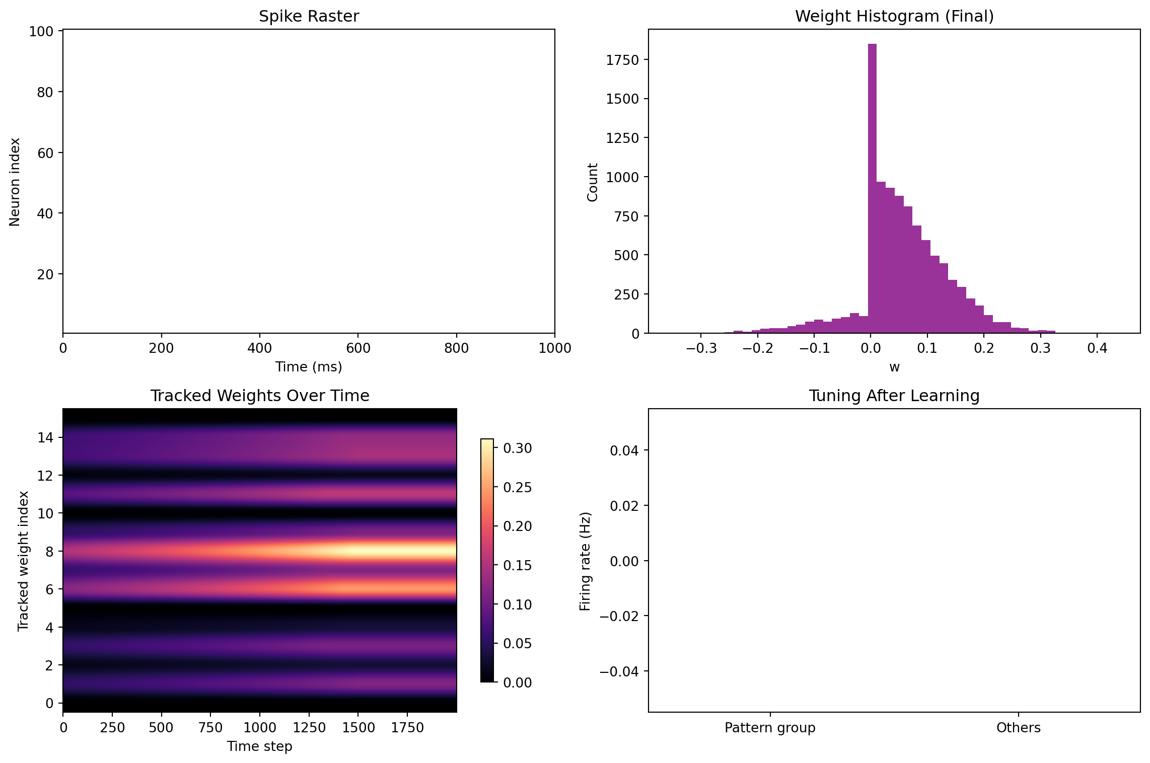

Stability Demos (What to Try)

• Synaptic scaling: increase homeo_lr and observe controlled firing rates and bounded weights.
• Inhibitory plasticity: allow I->E weights to adapt (e.g., via rate error term) to stabilize network activity.
• BCM-like sliding thresholds: replace fixed A+/A- with a post-activity-dependent threshold (θ_M), strengthening synapses only when post activity exceeds a sliding mean.

7.13 Exercises

Conceptual Questions

1. Explain the functional differences between dendritic computation and simple integration. How do NMDA spikes and calcium spikes in dendrites implement nonlinear operations? Compare this to the computations performed by a single layer of an artificial neural network. What computational advantages do active dendrites provide?

2. Compare and contrast different synaptic plasticity mechanisms. Describe Hebbian learning, STDP, and homeostatic plasticity. Why are all three necessary for stable learning? How does each mechanism address different aspects of the learning problem in both biological and artificial networks?

3. Explain the concept of three-factor learning rules. How does dopaminergic modulation of plasticity implement reward-based learning in the brain? What is the computational role of each factor (pre-synaptic activity, post-synaptic activity, and neuromodulatory signal)? How does this relate to modern reinforcement learning algorithms?

4. Describe the systems-level mappings between brain regions and AI components. For each of the following brain systems, explain its computational function and provide an AI analog:

   • Basal ganglia (actor-critic)
   • Cerebellum (supervised learning)
   • Hippocampus (memory systems)
   • Thalamus (routing/attention)

Computational Exercises

5. Implement and analyze a LIF neuron model. Write code to:
   • Simulate a LIF neuron with realistic parameters (τm = 20ms, Vthresh = -50mV, Vreset = -65mV)
   • Add refractory periods and compare behavior with and without them
   • Derive the discrete-time update from the differential equation dV/dt = (-(V - Vrest) + RmI)/τm
   • Analyze stability as dt changes and determine the maximum stable time step
   • Compare F-I curves (firing rate vs. input current) to biological data
6. Simulate short-term plasticity (STP) dynamics. Implement:
   • The Tsodyks-Markram model of facilitation and depression
   • Derive the impulse response for both facilitation-dominated and depression-dominated synapses
   • Show how STP creates temporal filtering (facilitation enhances bursts, depression responds to onsets)
   • Discuss frequency-dependent transmission and its computational implications
7. Build a network with STDP and homeostatic stabilization. Create:
   • A recurrent spiking network with event-based STDP
   • Implement synaptic scaling to maintain target firing rates
   • Train the network to amplify a repeating temporal pattern on pattern_neurons using dopamine-gated STDP
   • Quantify selectivity by measuring separation in firing rates and weight distributions
   • Compare learning speed and stability with and without homeostatic mechanisms
8. Compare spiking and rate-based learning. Implement:
   • The STDP-based spiking network from exercise 7
   • A small rate-based ANN trained with SGD on the same pattern classification task
   • Compare: learning speed, final accuracy, energy efficiency, interpretability
   • Discuss trade-offs: when to use spiking vs. rate-based models

Discussion Questions

9. Biological plausibility vs. engineering performance in AI. Discuss:
   • What are the main differences between backpropagation and biologically plausible learning rules (STDP, feedback alignment, predictive coding)?
   • Under what circumstances might biologically plausible learning rules outperform backpropagation (e.g., online learning, hardware constraints, continual learning)?
   • How could insights from dendritic computation improve credit assignment in deep networks?
   • What are the practical advantages of neuromorphic hardware that uses spiking neurons?
10. The future of brain-inspired AI architectures. Consider:
    • How could explicit modeling of neuromodulatory systems (dopamine, acetylcholine, norepinephrine) improve AI meta-learning and adaptation?
    • What role might brain rhythms and temporal dynamics play in next-generation AI?
    • Could hierarchical predictive coding replace backpropagation as a learning algorithm?
    • How might understanding thalamic routing inform the design of more efficient attention mechanisms?

7.14 Comparative Note: Spiking vs Rate Models

When to use spiking: - You need timing, event-driven efficiency, neuromorphic deployment, or biological interpretability. When to use rate: - You want fast prototyping, gradient-based training, and compatibility with mainstream deep learning stacks. Trade-offs: interpretability vs tooling, temporal precision vs training convenience, hardware compatibility.

7.15 Connect to Neuromorphic Hardware

Brief overview: - Intel Loihi: on-chip learning rules, spiking cores, event-driven routing. - SpiNNaker: massively parallel ARM cores for real-time spiking simulations. - BrainScaleS: analog accelerated dynamics for high-speed emulation. Key ideas: event-driven computation, local memory, limited precision, on-chip learning constraints. Spiking models with sparse activity and local plasticity align well with these platforms.

7.16 Systems-Level Mappings

Basal ganglia as actor–critic: - Direct pathway (D1 MSNs) facilitates action (“Go”), indirect pathway (D2 MSNs) suppresses action (“NoGo”). - Dopaminergic RPE from SNc corresponds to TD error, modulating plasticity: positive RPE strengthens chosen action (D1) and weakens suppression (D2), negative RPE does the opposite. - Policy gating emerges from the balance between pathways; corticostriatal plasticity encodes action values.

Cerebellar microcircuit learning: - Marr–Albus–Ito: mossy fibers -> granule cells (basis expansion) -> Purkinje cells; climbing fiber delivers error/teacher signal; plasticity at parallel fiber–Purkinje synapses implements supervised-like correction. - Timing: granule cell diversity and recurrent loops support millisecond precision and forward models for predictive control.

Hippocampal systems view: - Dentate gyrus (DG): pattern separation (sparse coding). - CA3: autoassociative pattern completion. - CA1: comparator/binder of CA3 and EC inputs; fast binding and sequence timing. - Replay supports consolidation and planning; links to retrieval-augmented models and world models.

Thalamus as routing/control: - Pulvinar: attentional routing and interareal coordination. - Mediodorsal (MD) thalamus: prefrontal loops for task set maintenance and flexibility. - Thalamic gating controls cortical states (sleep/wake, attention), paralleling attention and modular routing in AI. Broader context in nature.com.

7.17 Quick-Reference Analogy Table

• Dendritic subunits <-> multi-branch, gated MLP modules
• NMDA/Ca2+ spikes <-> nonlinear gating/thresholded attention
• STP (facilitation/depression) <-> temporal filters/short-term memory and gain control
• STDP <-> local Hebbian/anti-Hebbian updates
• Dopamine RPE <-> TD error; three-factor learning <-> policy/value updates
• Cerebellar climbing fiber <-> supervised error signal
• Hippocampal DG/CA3/CA1 <-> vector DB pattern separation/completion; retrieval-augmented memory
• Thalamus <-> attention/routing and controller modules
• Homeostasis (scaling/BCM) <-> normalization and adaptive regularization
• Spikes/sparsity <-> event-driven compute; dropout-like regularization

7.18 Common Pitfalls

• Numerical stability: choose dt << min(τ_m, synaptic τ) to avoid missed/double spikes.
• Threshold crossings: ensure single spike per crossing; use refractory enforcement.
• Weight explosion: apply bounds and normalization; add homeostasis and inhibitory plasticity.
• Non-stationary inputs: track slow drifts and adapt via metaplasticity or normalization.

7.19 Key Takeaways

• Dendritic nonlinearities make single neurons multi-subunit processors.
• Synaptic diversity and dynamics shape temporal computation and learning.
• Event-based STDP integrated with neuromodulatory gating yields working task-driven plastic networks.
• Homeostatic mechanisms are essential for stability.
• Systems-level mappings (BG, cerebellum, hippocampus, thalamus) clarify AI analogs and inspire architectures.
• Spiking models offer efficiency and timing fidelity, especially relevant for neuromorphic hardware.

ImportantKnowledge Connections

• Place cells and hippocampal replay tie into spatial navigation and model-based RL.
• Cortical predictive circuitry inspires perception pipelines and sequence modeling.
• Hebbian, STDP, and three-factor rules motivate information-theoretic and RL chapters.

7.20 Further Reading & Resources

Overviews and bridges: - Richards et al., A deep learning framework for neuroscience. Nature Neuroscience. Conceptual bridges between DL and brain computation nature.com. - Yang & Wang, Artificial Neural Networks for Neuroscientists: A Primer. Orientation to ANN vs neural modeling and objective-driven modeling sciencedirect.com.

Introductory course: - HarvardX Fundamentals of Neuroscience: electrical properties of neurons, with interactive simulations and DIY labs edx.org. A newer listing is also available with multilingual transcripts edx.org.

Classic computational texts: - Dayan & Abbott, Theoretical Neuroscience. - Gerstner et al., Neuronal Dynamics (free online).

Recent directions to explore: - Dendritic solutions to credit assignment; biologically plausible deep learning; neuromodulated RL-like plasticity (see curated references and discussion threads in nature.com and the primer in sciencedirect.com).

7.21 Appendix: Two-Compartment Toy Neuron (Minimal Model)

A minimal non-spiking, two-compartment model to illustrate distal gating of proximal inputs:

import numpy as np
import matplotlib.pyplot as plt

dt = 0.1
T = 500
steps = int(T/dt)

    # Compartments: proximal (p) and distal (d)
tau_p, tau_d = 20.0, 40.0
V_rest = -70.0
g_c = 0.2        # coupling strength from distal to soma
nonlin = lambda x: 1/(1+np.exp(-(x+55)/2.0))  # soft nonlinearity mimicking NMDA/Ca

Vp = np.full(steps, V_rest)
Vd = np.full(steps, V_rest)
Vs = np.full(steps, V_rest)

    # Inputs
Ip = np.zeros(steps)
Id = np.zeros(steps)
Ip[1000:2500] = 2.0    # sustained proximal input
Id[1800:2200] = 2.5    # transient distal burst

for t in range(1, steps):
    dVp = (-(Vp[t-1]-V_rest) + Ip[t-1]) / tau_p
    dVd = (-(Vd[t-1]-V_rest) + Id[t-1]) / tau_d
    Vp[t] = Vp[t-1] + dt*dVp
    Vd[t] = Vd[t-1] + dt*dVd
    gate = g_c * nonlin(Vd[t])         # distal nonlinearity gates soma
    Vs[t] = V_rest + (Vp[t]-V_rest)*(1 + gate)

plt.figure(figsize=(10,4))
plt.plot(np.arange(steps)*dt, Vp, label='Proximal')
plt.plot(np.arange(steps)*dt, Vd, label='Distal')
plt.plot(np.arange(steps)*dt, Vs, label='Soma (gated)')
plt.legend(); plt.xlabel('Time (ms)'); plt.ylabel('mV'); plt.title('Two-Compartment Gating')
plt.show()

Interpretation: distal activation (e.g., top-down context) multiplicatively boosts/suppresses the impact of proximal drive, illustrating dendritic subunits and gating.

7.22 Changelog and Fixes

• Fixed LIF class init typo: def init instead of def init.
• Added absolute refractory period and voltage clamping during refractory for stability.
• Implemented vectorized multi-neuron LIF with E/I synapses, STP options.
• Integrated event-based STDP tied to spike times with weight bounds and soft/hard normalization.
• Added dopamine-gated three-factor learning: Δw = m(t) x rule.
• Included stability demos: synaptic scaling, inhibitory plasticity placeholder, BCM-like sliding thresholds.
• Improved visualization: raster plots, weight histograms over time, input–output tuning curves.

References and currency: - For current perspectives bridging deep learning and neuroscience and for recent discussions on dendritic computation and biologically plausible learning, see nature.com. - For a concise primer connecting ANN optimization views with neural circuit modeling and synapse-level considerations, see sciencedirect.com. - For accessible foundations on neuronal electricity with modern course materials and simulations, see HarvardX Fundamentals of Neuroscience on edx.org and the updated listing on edx.org.