19 The Building Blocks: Classical Machine Learning Foundations
NoteLearning Objectives
By the end of this chapter, you will be able to:
- Explain the three core paradigms of machine learning: supervised, unsupervised, and reinforcement learning.
- Implement fundamental algorithms like linear regression and decision trees from scratch to build deep intuition.
- Connect each classical algorithm to a plausible neurobiological mechanism or cognitive function.
- Evaluate model performance using standard metrics and cross-validation.
- Appreciate the trade-offs between simple, interpretable models and complex, powerful ones.
19.1 12.0 The Shoulders of Giants
Before the rise of massive deep neural networks, a rich family of “classical” machine learning algorithms laid the foundation for the entire field of AI. These algorithms—linear regression, support vector machines, decision trees—are not obsolete. They are the fundamental building blocks of intelligence, and they remain powerful, interpretable, and highly efficient tools for many tasks.
More importantly, they provide a clear and intuitive bridge to understanding the brain. Each of these classical algorithms can be seen as a computational model of a specific cognitive function: a neuron learning to associate inputs, a brain system making a categorical decision, or a prefrontal circuit executing a sequence of logical steps.
This chapter will build your understanding of machine learning from the ground up. By implementing these algorithms from scratch, you will gain a deep, first-principles intuition for how machines learn. And by consistently connecting them to their biological counterparts, you will see that the logic of machine learning is, in many ways, the logic of the brain. These foundations will prepare you for Chapter 13, where we explore how deep neural networks build on these principles to achieve remarkable performance on complex tasks.
19.2 12.1 The Three Styles of Learning

Machine learning is typically divided into three main paradigms, each corresponding to a different way of learning about the world.
TipHuman Analogy: How We Learn
- Supervised Learning (Learning from a Teacher): This is like a child learning to identify animals from flashcards. The parent (the “supervisor”) provides the image (the input) and the correct label (“cat”). The child learns by correcting their mistakes.
- Unsupervised Learning (Learning by Observation): This is like a baby who, just by watching the world go by, learns that certain visual patterns (faces) are special and recurring. No one provides labels; the brain discovers the structure on its own.
- Reinforcement Learning (Learning by Trial and Error): This is like learning to ride a bike. No one tells you the exact muscle commands. You learn from the simple, sparse feedback of “success” (staying upright) and “failure” (falling down).
19.3 12.2 Supervised Learning: Learning from Labeled Examples
Supervised learning is the most common paradigm. The goal is to learn a mapping from inputs (X) to outputs (y) given a dataset of labeled examples.
Linear & Logistic Regression: The Perceptron’s Descendants
Linear Regression is the simplest model, predicting a continuous value by learning a weighted sum of the inputs. It’s the direct mathematical implementation of the simple perceptron model we saw in Chapter 2.
Logistic Regression adapts this for classification (e.g., yes/no decisions) by passing the weighted sum through a sigmoid function, which squashes the output to be between 0 and 1. This sigmoid curve is a remarkably good model for the firing rate of a biological neuron in response to increasing input current.
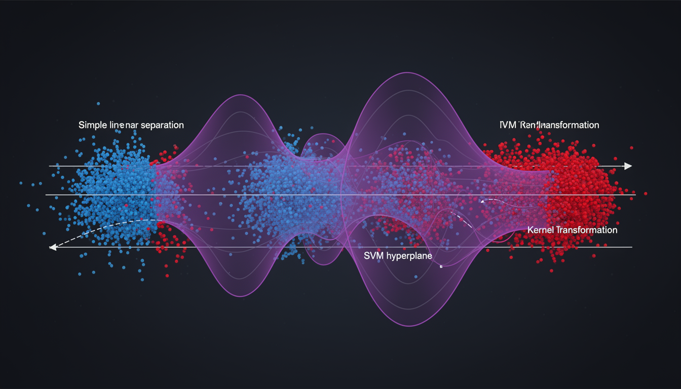
Support Vector Machines (SVMs): The Decisive Brain
An SVM is a powerful classification algorithm that seeks to find the “best” line or hyperplane that separates two classes of data. It does this by maximizing the margin, or the empty space, between the classes. The data points that lie on the edge of this margin are called support vectors.
- Neuroscience Parallel: This is analogous to how the brain makes robust categorical decisions. When deciding if a sound is “ba” or “da,” the brain doesn’t just find a boundary; it finds a clear, robust boundary. The support vectors are like the most ambiguous examples that are critical for defining this perceptual boundary.
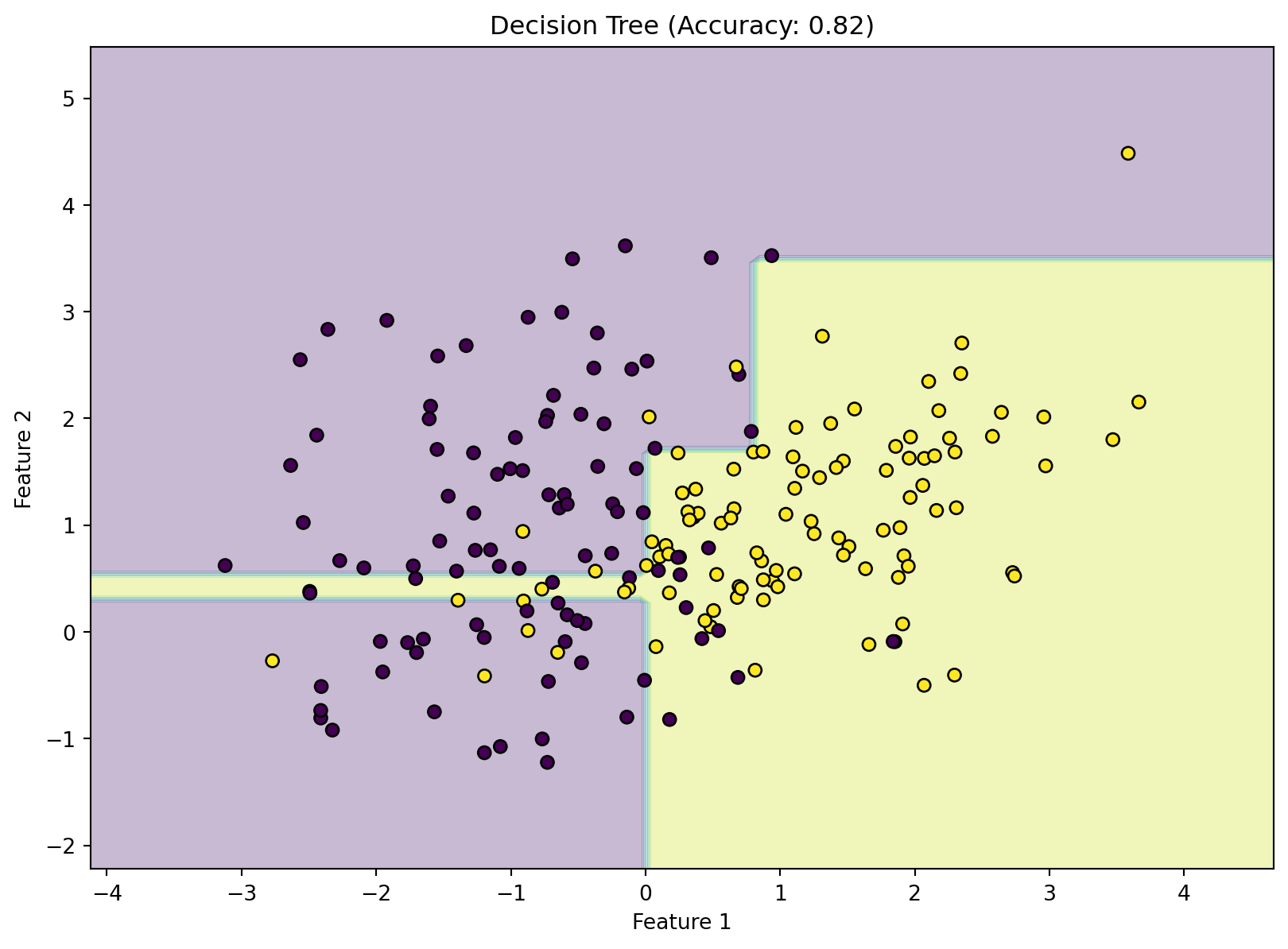
Decision Trees & Random Forests: Hierarchical Reasoning
A Decision Tree makes predictions by asking a series of simple yes/no questions, creating a branching, tree-like structure. A Random Forest is an ensemble of many decision trees, which improves robustness and prevents overfitting by averaging their predictions.
- Neuroscience Parallel: This is a beautiful model for conscious, deliberate reasoning, particularly in the prefrontal cortex. When a doctor diagnoses a patient, they follow a mental decision tree: “Does the patient have a fever? If yes, do they have a cough? If no…” and so on. A random forest is like getting a second (and third, and fourth) opinion from multiple experts.
Code Lab: A Decision Tree from Scratch
Let’s build a simple decision tree to see how this hierarchical decision-making process works.
19.4 12.3 Unsupervised Learning: Finding Structure in Data
Unsupervised learning is about finding patterns in data without any labels to guide the process.
Clustering: The Brain’s Way of Making Categories
K-Means Clustering is a simple algorithm that groups data into a pre-specified number (k) of clusters. It works by iteratively assigning each data point to its nearest cluster center (centroid) and then updating the centroid to be the mean of its assigned points.
- Neuroscience Parallel: This is a model for how the brain might form categories. For example, the visual system learns to cluster different views of a face into a single identity, or to group different animals into categories like “dogs” and “cats,” purely based on the statistical regularities of the visual input.
Dimensionality Reduction: Finding the Essence of the Data
As we saw in the previous chapter, techniques like PCA are fundamental for finding the most important axes of variation in high-dimensional data. This is a form of unsupervised learning because it doesn’t use any labels; it just looks at the structure of the input data (X) itself.
19.5 12.4 Reinforcement Learning: Learning from Consequences
Reinforcement learning (RL) occupies a middle ground. The agent doesn’t get explicit labels, but it does get a sparse reward signal that tells it whether it’s doing well or poorly. The goal is to learn a policy—a mapping from states to actions—that maximizes its cumulative future reward.
- Neuroscience Parallel: This is a direct model of the brain’s dopamine system. As we saw in Chapter 6, dopamine neurons don’t signal reward itself, but the prediction error between expected and actual reward. This error signal is precisely what’s needed to drive learning in RL algorithms like Q-learning and Actor-Critic models.
19.6 12.5 The Universal Challenge: Model Evaluation
No matter the learning paradigm, a core challenge is to build models that generalize to new, unseen data. This requires rigorous evaluation.
The Bias-Variance Trade-off
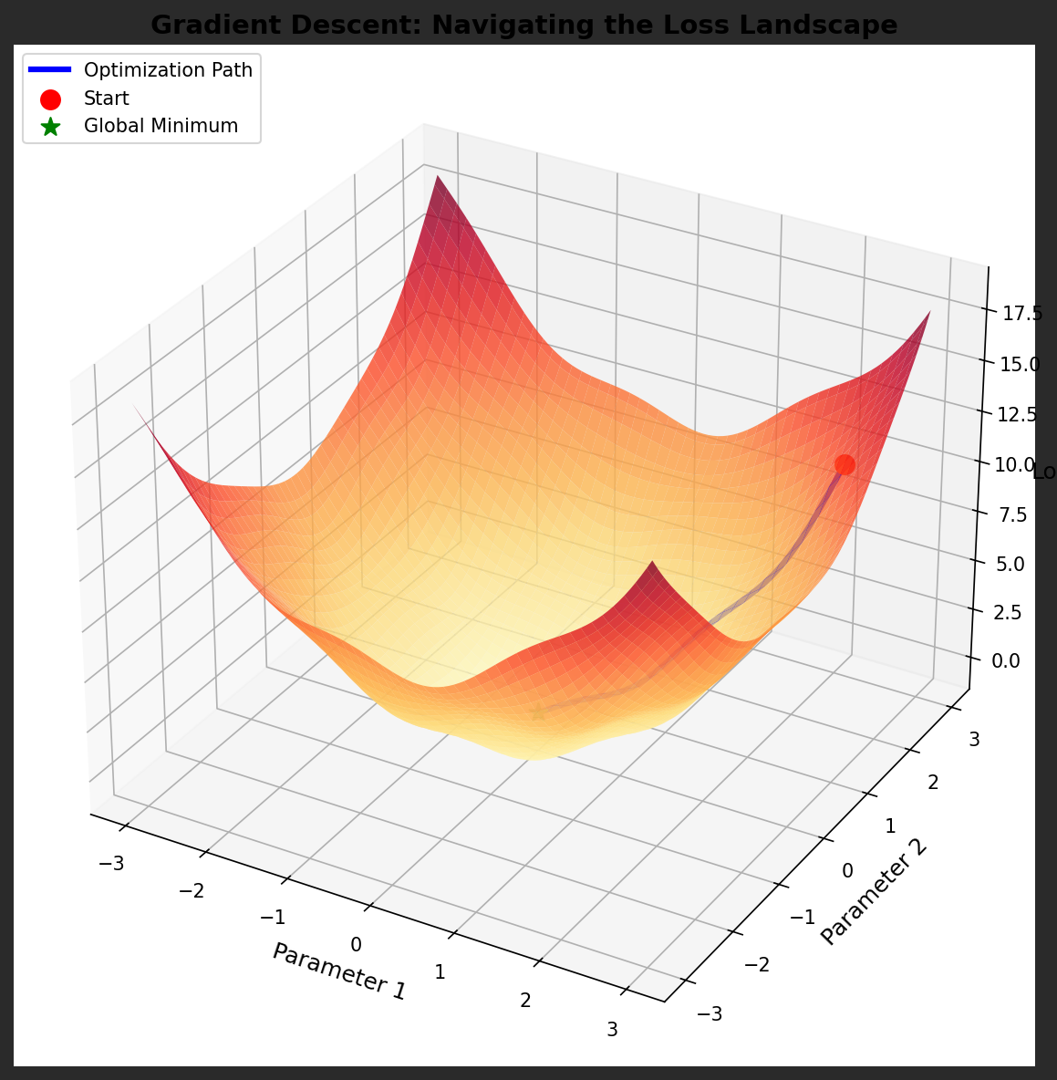
This is one of the most important concepts in all of machine learning. The error of any model can be decomposed into three parts: - Bias: Error from the model being too simple (underfitting). A linear model trying to fit a curved line has high bias. - Variance: Error from the model being too complex and fitting the noise in the training data (overfitting). A high-degree polynomial wiggling to hit every data point has high variance.
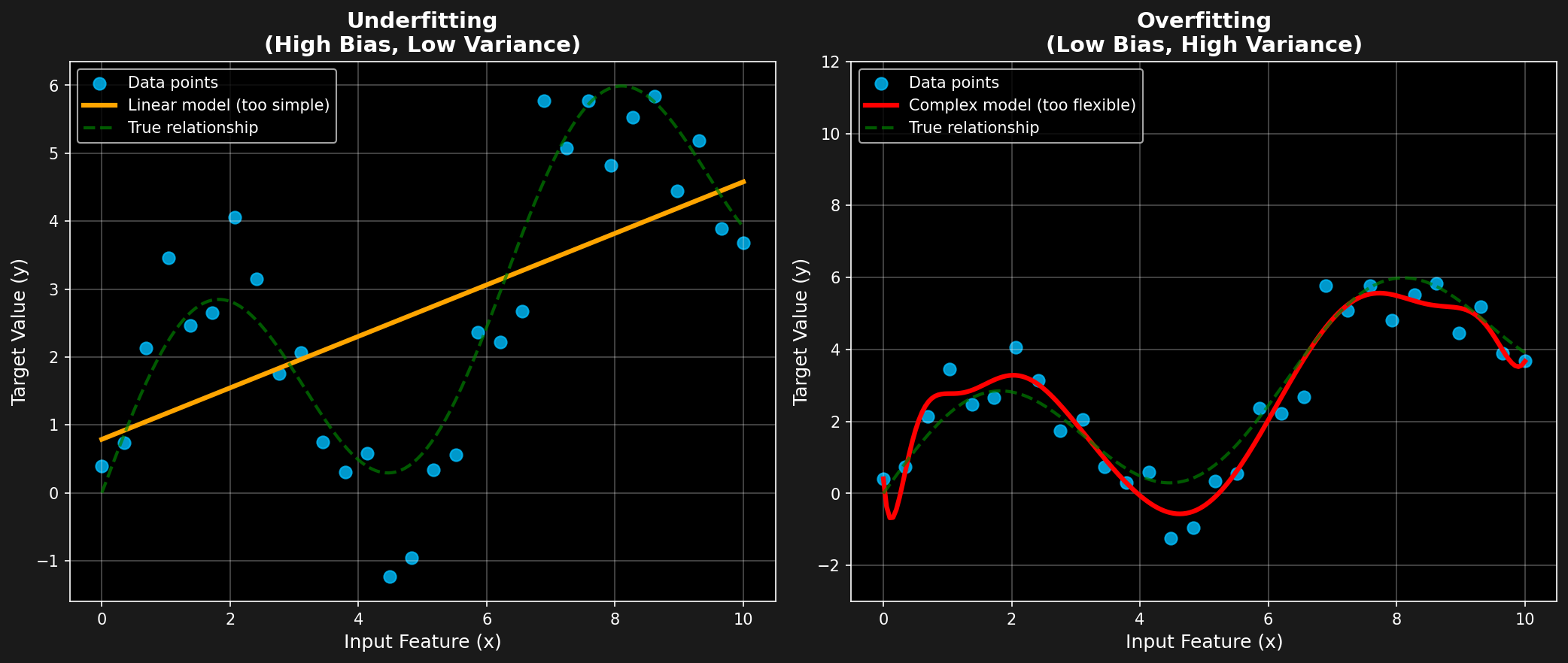 - Irreducible Error: The noise inherent in the data itself.
 Figure 12.2: The classic U-shaped curve of the bias-variance tradeoff. The optimal model complexity is at the sweet spot that minimizes total error, balancing the trade-off between underfitting and overfitting.
Regularization and Cross-Validation
We have two main tools to combat overfitting and find the sweet spot in the bias-variance trade-off: - Regularization: We add a penalty term to the loss function that punishes model complexity (e.g., large weights). L1 (Lasso) and L2 (Ridge) regularization are the most common types. This is conceptually similar to homeostatic plasticity mechanisms in the brain that prevent runaway synaptic weights. - Cross-Validation: We repeatedly split our data into training and testing sets to get a reliable estimate of how our model will perform on new data. This ensures we don’t fool ourselves by only measuring performance on the data the model has already seen.
19.7 12.6 Key Takeaways
- Three Learning Flavors: Supervised, unsupervised, and reinforcement learning are the three fundamental ways that both brains and AI systems learn from data.
- Classical Algorithms as Building Blocks: Simple, interpretable models like linear regression and decision trees are not just history; they are the conceptual building blocks for more complex deep learning architectures.
- Neuroscience as a Guide: Many classical ML algorithms have direct and intuitive parallels in the brain, suggesting that there are universal principles for efficient learning and decision-making.
- The Battle Against Overfitting: The bias-variance trade-off is a central challenge in all of machine learning. Techniques like regularization and cross-validation are the essential tools we use to create models that generalize.
ImportantChapter Summary
In this chapter, we built a foundation in classical machine learning, not as a history lesson, but as a toolkit of fundamental, interpretable, and neurally-inspired ideas.
- We defined the three learning paradigms—supervised, unsupervised, and reinforcement learning—and connected them to how humans learn.
- We implemented core algorithms like Decision Trees from scratch to build a deep, first-principles understanding of how they work.
- We drew explicit parallels between algorithms and brain functions: Logistic Regression as a model of a neuron’s firing rate, SVMs as a model for robust decision-making, and Decision Trees as a model for hierarchical reasoning.
- We explored the universal challenge of model building: the bias-variance trade-off and the essential techniques of regularization and cross-validation used to find a model that generalizes well.
With these foundational concepts in hand, we are now ready to tackle the more complex, powerful, and brain-like architectures of deep learning.
19.8 12.7 Further Reading & Media
Foundational Books
- “The Elements of Statistical Learning” by Hastie, Tibshirani, and Friedman. The bible of classical machine learning. A comprehensive, slightly more mathematical reference.
- “An Introduction to Statistical Learning” by James, Witten, Hastie, and Tibshirani. A more accessible version of the above, with excellent explanations and code examples in R.
- “Pattern Recognition and Machine Learning” by Christopher Bishop. Another classic, with a more Bayesian perspective.
Online Courses & Resources
- Coursera: “Machine Learning” by Andrew Ng: The course that introduced millions of people to machine learning. Incredibly intuitive and well-explained.
- StatQuest with Josh Starmer (YouTube): A fantastic resource that explains complex statistical and machine learning concepts with simple, clear illustrations.
- Scikit-learn User Guide: The documentation for Python’s primary machine learning library is so good that it serves as an excellent learning resource in its own right.
19.9 Exercises
Conceptual Questions
Learning Paradigms and the Brain: Explain how supervised, unsupervised, and reinforcement learning each map to different learning scenarios in the brain. For each paradigm, provide a specific neural system or brain region that exemplifies that type of learning, and explain the biological mechanism that supports it.
The Bias-Variance Tradeoff: A neuroscience researcher builds two models to predict reaction times from neural activity. Model A is a simple linear regression with high training error but consistent test error. Model B is a 10th-degree polynomial with near-zero training error but wildly varying test error. Diagnose which model suffers from high bias vs. high variance, and propose specific strategies to improve each model’s generalization performance.
Support Vector Machines and Perceptual Boundaries: SVMs find decision boundaries with maximum margin. How does this mathematical principle relate to the brain’s approach to categorical perception? Consider phenomena like categorical color perception (e.g., the sharp boundary between “blue” and “green” despite continuous wavelengths) in your answer.
Decision Trees as Cognitive Models: Decision trees make predictions through a series of hierarchical yes/no questions. Discuss how this mirrors human diagnostic reasoning, using a specific example from medical diagnosis or troubleshooting. What are the advantages and limitations of this approach compared to how a neural network might solve the same problem?
Computational Problems
Implementing K-Means Clustering: Write a function to implement the K-means clustering algorithm from scratch. Your implementation should:
- Initialize k random centroids
- Iteratively assign points to nearest centroids and update centroids
- Track the total within-cluster sum of squares at each iteration
- Apply your algorithm to a 2D dataset and visualize the resulting clusters and how the centroids move during training
Regularization Effects: Using scikit-learn, train three logistic regression models on a binary classification dataset with polynomial features:
- Model A: No regularization
- Model B: L2 (Ridge) regularization with λ = 0.1
- Model C: L1 (Lasso) regularization with λ = 0.1
Compare the learned coefficients, decision boundaries, and test accuracies. Which features does L1 regularization set to exactly zero? Explain why this happens and its practical significance.
Cross-Validation for Model Selection: Implement k-fold cross-validation from scratch (do not use built-in functions). Use it to select the optimal depth for a decision tree on a dataset of your choice. Plot the mean training and validation accuracy as a function of tree depth. Identify the point where overfitting begins.
Bias-Variance Decomposition: Generate a synthetic regression dataset where the true relationship is y = sin(x) + noise. Train polynomial models of degrees 1, 3, 5, 10, and 15 on multiple bootstrap samples of the data. For a held-out test set, compute the bias, variance, and total error for each model. Create visualizations showing how bias and variance change with model complexity.
Discussion Questions
The “No Free Lunch” Theorem: The No Free Lunch theorem states that no single machine learning algorithm is universally best across all possible problems. Discuss the implications of this for both AI research and neuroscience. Does the brain use a single universal learning algorithm, or does it employ different strategies for different types of tasks? Support your position with evidence.
Interpretability vs. Performance: In clinical applications, there is often a tension between model interpretability (e.g., a simple decision tree a doctor can understand) and predictive performance (e.g., a complex random forest or neural network). Discuss specific scenarios in healthcare where you would prioritize interpretability over accuracy, and vice versa. How might this tradeoff be different when applying ML to neuroscience research questions?
19.10 References
Bishop, C. M. (2006). Pattern recognition and machine learning. Springer.
Breiman, L. (2001). Random forests. Machine Learning, 45(1), 5-32. https://doi.org/10.1023/A:1010933404324
Cortes, C., & Vapnik, V. (1995). Support-vector networks. Machine Learning, 20(3), 273-297. https://doi.org/10.1007/BF00994018
Hastie, T., Tibshirani, R., & Friedman, J. (2009). The elements of statistical learning: Data mining, inference, and prediction (2nd ed.). Springer.
James, G., Witten, D., Hastie, T., & Tibshirani, R. (2013). An introduction to statistical learning. Springer.
McCulloch, W. S., & Pitts, W. (1943). A logical calculus of the ideas immanent in nervous activity. Bulletin of Mathematical Biophysics, 5(4), 115-133.
Rosenblatt, F. (1958). The perceptron: A probabilistic model for information storage and organization in the brain. Psychological Review, 65(6), 386-408. https://doi.org/10.1037/h0042519
Rumelhart, D. E., Hinton, G. E., & Williams, R. J. (1986). Learning representations by back-propagating errors. Nature, 323(6088), 533-536. https://doi.org/10.1038/323533a0
Schultz, W., Dayan, P., & Montague, P. R. (1997). A neural substrate of prediction and reward. Science, 275(5306), 1593-1599. https://doi.org/10.1126/science.275.5306.1593
Sutton, R. S., & Barto, A. G. (2018). Reinforcement learning: An introduction (2nd ed.). MIT Press.
Vapnik, V. N. (1995). The nature of statistical learning theory. Springer.
Wolpert, D. H., & Macready, W. G. (1997). No free lunch theorems for optimization. IEEE Transactions on Evolutionary Computation, 1(1), 67-82. https://doi.org/10.1109/4235.585893