22 Sequence Models: RNN -> Attention -> Transformer
NoteLearning Objectives
By the end of this chapter, you will be able to:
- Understand how text is segmented and preprocessed for neural models
- Connect tokenization to the brain’s mechanisms for segmenting continuous speech
- Master classical NLP preprocessing: stemming, lemmatization, and text vectorization
- Understand the evolution of sequence models from RNNs to Transformers
- Master the architectures and training methods for recurrent networks, attention mechanisms, and transformer models
- Connect sequence model operations to temporal processing in the brain
- Implement key sequence modeling architectures for various tasks
- Compare different approaches to handling sequential data
- Apply sequence models to healthcare time series data for clinical applications
- Address challenges unique to healthcare sequences such as irregularity and missing data
22.1 14.0 Text Processing Fundamentals: From Sounds to Symbols
Before neural networks can process language, text must be transformed into numerical representations. This preprocessing pipeline, often overlooked in discussions of modern AI, draws on insights from linguistics, information theory, and remarkably, from how the human brain itself segments continuous speech into discrete units.
14.0.1 The Word Segmentation Problem
What is a word? This seemingly simple question is surprisingly difficult to answer. Consider the spoken sentence “I saw a caterpillar.” When you hear it, there are no pauses between words. There is just a continuous stream of sound. Yet your brain effortlessly segments this acoustic signal into four distinct units.
TipNeuroscience Connection: How the Brain Segments Speech
The human auditory system faces a computational challenge identical to what computers face when processing text without spaces. Continuous speech contains no reliable acoustic markers for word boundaries. The pauses we “hear” between words are largely a cognitive illusion constructed by our brains.
Research in psycholinguistics reveals that infants learn to segment speech using statistical regularities: - Transitional probabilities: The syllable “pre” is often followed by “tty” in “pretty,” but “ty” rarely leads to “ba.” Infants as young as 8 months track these statistics to identify word boundaries. - Prosodic cues: Stress patterns, pitch contours, and vowel lengthening provide hints about word structure. - Phonotactic constraints: Some sound combinations are illegal within words (e.g., “ng” can end but not begin English words), signaling boundaries.
The brain’s superior temporal sulcus and Broca’s area form a network that integrates these cues in real-time at roughly 150 milliseconds per word, a feat that modern NLP systems approximate through tokenization algorithms.
Interestingly, the challenge of word segmentation isn’t just a modern computational problem. Ancient written languages often lacked the conventions we take for granted:
- Scriptio continua: Latin and Greek texts were written without spaces between words: INTHEBEGINNINGWASTHEWORD
- No punctuation: Periods, commas, and other markers were later inventions
- No lowercase: The distinction between uppercase and lowercase emerged in medieval manuscripts
Reading such texts required significant cognitive effort, exactly the same effort computers must expend today when processing raw text streams. The solution in both cases involves pattern recognition, context, and learned statistical regularities.
14.0.2 Words, Tokens, and Morphemes
Modern NLP distinguishes several units of text:
Word Types vs. Word Instances Consider the sentence: “The cat sat on the mat.” This contains 6 word instances (also called tokens) but only 5 unique word types (since “the” appears twice). The relationship between types and instances follows a remarkable pattern:
- Zipf’s Law: Word frequency follows a power law distribution. In English, “the” alone accounts for about 7% of all words. The 100 most common words cover roughly half of all text.
- Heaps’ Law (also called Herdan’s Law): Vocabulary size grows sublinearly with corpus size. If \(|V|\) is vocabulary size and \(N\) is the number of tokens, then \(|V| = kN^\beta\) where \(\beta \approx 0.5-0.7\).
This means a corpus of 1 million words might have 30,000 unique word types, while a corpus of 1 billion words might have only 500,000. Vocabulary grows, but ever more slowly.
Morphemes: The Atoms of Meaning Words themselves are built from smaller meaning-bearing units called morphemes:
- Stems: The core meaning unit (e.g., “walk” in “walking”)
- Affixes: Prefixes and suffixes that modify meaning
- Derivational morphemes create new words: “un-” + “happy” → “unhappy”
- Inflectional morphemes modify grammatical function: “walk” + “-ed” → “walked”
The English word “unlikeliest” contains four morphemes: un- + like + -ly + -est. Understanding morphology is crucial because: 1. It explains why “walking,” “walked,” and “walks” should be related 2. It motivates stemming and lemmatization algorithms 3. It underlies modern subword tokenization (like BPE)
TipNeuroscience Connection: Morphological Processing in the Brain
Neuroimaging studies reveal that the brain processes morphologically complex words differently from simple ones. When reading “unhappiness”: - The visual word form area (left fusiform gyrus) initially processes the whole string - Broca’s area and surrounding regions decompose it into morphemes - Semantic areas integrate the meaning of the components
Priming experiments show that seeing “walked” speeds recognition of “walk,” suggesting that morphological decomposition is automatic. This biological insight inspired computational approaches that break words into meaningful subunits rather than treating each word form as entirely distinct.
14.0.3 Classical Text Preprocessing
Before the neural network revolution, text preprocessing involved a series of explicit transformations. While modern LLMs handle many of these implicitly, understanding the classical pipeline remains valuable.
Tokenization Tokenization segments text into discrete units. For English, this seems trivial: split on whitespace and punctuation. But edge cases abound:
- Contractions: Is “don’t” one token or two (“do” + “n’t”)?
- Hyphenated words: “state-of-the-art” = 1 word or 4?
- Abbreviations: “Dr.” includes a period that isn’t sentence-ending
- Numbers: Should “3.14” be split at the decimal?
- URLs and emails: “[email protected]” shouldn’t be split
Different tokenizers make different choices, and these decisions ripple through downstream processing.
Normalization Raw text contains variations that may or may not be meaningful:
- Case folding: Converting “Apple” and “apple” to the same form (but losing the distinction between the company and the fruit)
- Unicode normalization: The character “é” can be represented as a single codepoint or as “e” + combining accent mark
- Punctuation handling: Removing or standardizing quotes, dashes, and other marks
Stemming and Lemmatization Both techniques reduce words to base forms, but with different philosophies:
Stemming: Crude rule-based chopping of suffixes. The Porter Stemmer converts “running,” “runs,” and “ran” all to “run” by applying rules like “if word ends in ‘ing’ and has a vowel before it, remove ‘ing’.” Stemming is fast but can produce non-words (“studies” → “studi”).
Lemmatization: Using vocabulary and morphological analysis to find the dictionary form. “Better” lemmatizes to “good” (its lemma), which stemming cannot achieve. Lemmatizers use part-of-speech information: “saw” lemmatizes to “see” (verb) or “saw” (noun) depending on context.
Stop Words Function words like “the,” “is,” “at,” and “which” occur frequently but carry little semantic content on their own. Classical approaches often removed these stop words to focus on content-bearing terms.
However, this practice has declined because: 1. Stop words carry grammatical information (compare “what is it” vs. “it is what”) 2. Modern models have the capacity to learn what to ignore 3. Some queries depend on stop words (“to be or not to be”)
14.0.4 From Words to Vectors: Representations for Machines
Computers require numerical input, so text must be converted to vectors. This transformation is fundamental to all neural NLP.
One-Hot Encoding The simplest approach assigns each word a unique index and represents it as a vector of all zeros except for a single 1 at that index. For a vocabulary of 50,000 words, each word becomes a 50,000-dimensional vector.
Problems: - Dimensionality: Vectors are enormous and sparse - No similarity: “cat” and “dog” are just as different as “cat” and “refrigerator” - No generalization: The model cannot use knowledge about “cat” when processing “feline”
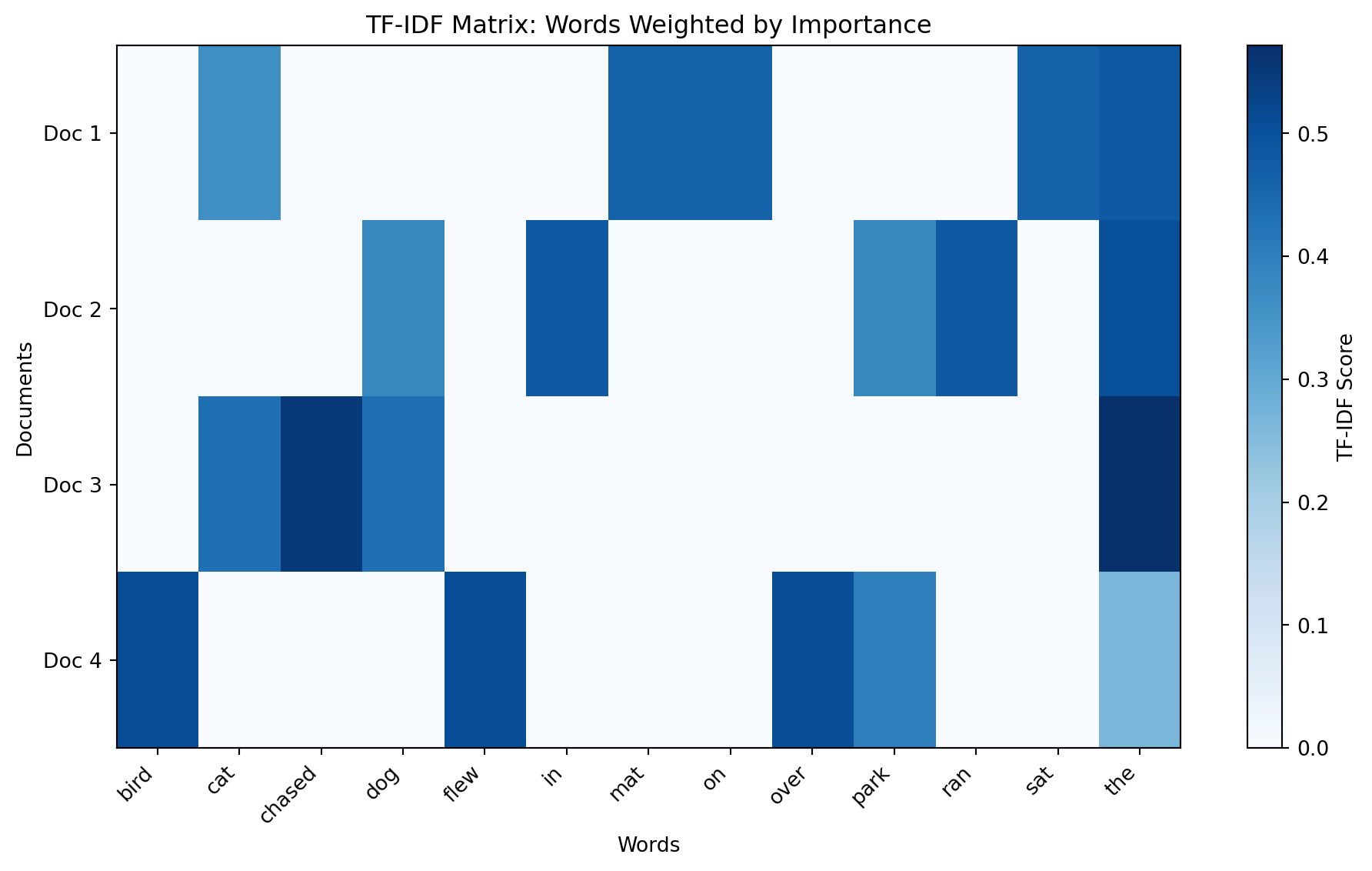
TF-IDF: Term Frequency–Inverse Document Frequency This classical method represents documents (not individual words) as vectors where each dimension corresponds to a word in the vocabulary:
\[\text{TF-IDF}(t, d, D) = \text{TF}(t, d) \times \text{IDF}(t, D)\]
- TF (Term Frequency): How often word \(t\) appears in document \(d\)
- IDF (Inverse Document Frequency): \(\log(N / n_t)\) where \(N\) is total documents and \(n_t\) is documents containing \(t\)
Words that appear frequently in one document but rarely across the corpus get high scores. This remains useful for document retrieval and as a baseline.
Word Embeddings: The Neural Revolution The breakthrough came with learning dense, distributed representations where semantically similar words have similar vectors. Word2Vec, GloVe, and FastText learn embeddings such that:
- Vector(“king”) - Vector(“man”) + Vector(“woman”) ≈ Vector(“queen”)
- Synonyms cluster together in embedding space
- Dimensions encode latent semantic features
These embeddings, typically 100-300 dimensions, capture rich semantic relationships learned from co-occurrence patterns in large corpora. They form the input layer for the neural sequence models we explore next.
14.0.5 N-gram Language Models: The Statistical Foundation
Before neural networks dominated NLP, n-gram language models were the workhorse of language modeling. Understanding them is essential because they reveal both the core problem that language models solve and why neural approaches were such a breakthrough.
The Language Modeling Task
A language model assigns probabilities to sequences of words. Given a sentence, it answers: “How likely is this sequence?” More practically, it can predict the next word given the previous context:
\[P(w_n | w_1, w_2, ..., w_{n-1})\]
This simple capability underlies spell-checking, speech recognition, machine translation, and (as we’ll see) modern chatbots.
The Markov Assumption
Computing the exact probability \(P(w_n | w_1, ..., w_{n-1})\) requires knowing the joint distribution of all possible word sequences, an impossibly large space. N-gram models make a Markov assumption: the probability of a word depends only on the previous \(n-1\) words.
- Unigram (\(n=1\)): \(P(w_i)\), where each word is independent
- Bigram (\(n=2\)): \(P(w_i | w_{i-1})\), depends on previous word only
- Trigram (\(n=3\)): \(P(w_i | w_{i-2}, w_{i-1})\), depends on two previous words
For a bigram model, the probability of a sentence is:
\[P(\text{"the cat sat"}) = P(\text{the}) \times P(\text{cat}|\text{the}) \times P(\text{sat}|\text{cat})\]
These probabilities are estimated by counting occurrences in a large corpus:
\[P(w_i | w_{i-1}) = \frac{\text{Count}(w_{i-1}, w_i)}{\text{Count}(w_{i-1})}\]
TipNeuroscience Connection: Predictive Processing in Auditory Cortex
The brain operates as a prediction machine, and this is vividly demonstrated in language processing. When you hear “peanut butter and…”, your auditory cortex doesn’t passively wait. It pre-activates neurons representing likely continuations like “jelly” before the word arrives.
This was elegantly demonstrated using MEG (magnetoencephalography) by Federenko and colleagues: brain activity patterns for highly predictable words begin forming 200-400ms before the word is even heard. The brain is essentially running its own language model, making n-gram-like predictions based on context.
When an unexpected word arrives (high surprisal), the brain generates a characteristic N400 event-related potential, a neural “prediction error” signal that drives learning. This is strikingly analogous to how n-gram models assign low probability to unexpected continuations.
Evaluating Language Models: Perplexity
How do we measure if a language model is good? The standard metric is perplexity, which measures how “surprised” the model is by test data:
\[\text{Perplexity}(W) = P(w_1, w_2, ..., w_N)^{-1/N} = \sqrt[N]{\frac{1}{P(w_1, w_2, ..., w_N)}}\]
Perplexity can be interpreted as the weighted average branching factor, indicating how many words the model considers equally likely at each position. Lower is better:
- Perplexity = 1: Perfect prediction (only one possible next word)
- Perplexity = 100: On average, 100 words are equally likely
- Perplexity = V (vocabulary size): No better than random guessing
Perplexity is directly related to cross-entropy loss, the standard training objective for neural language models:
\[\text{Perplexity} = 2^{\text{Cross-Entropy}}\]
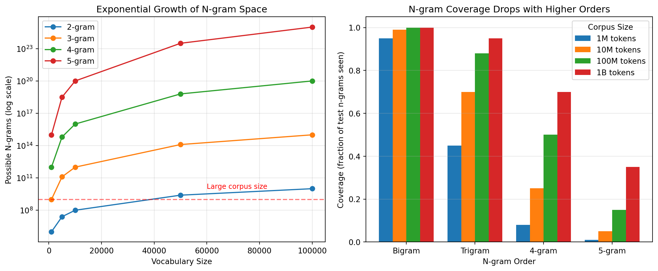
The Curse of Dimensionality: Why N-grams Fail
N-gram models face a fundamental problem: sparsity. Consider a trigram model with a vocabulary of 50,000 words. The number of possible trigrams is \(50,000^3 = 125\) trillion. No corpus is large enough to observe most of these combinations even once.
This creates two devastating problems:
Zero probabilities: Any unseen n-gram gets \(P = 0\), making entire sentences impossible. If “quantum computing” never appeared in training, \(P(\text{computing}|\text{quantum}) = 0\).
No generalization: The model cannot use the similarity between “cat” and “dog” to transfer knowledge. Seeing “the cat sat” tells it nothing about “the dog sat.”
Smoothing techniques (Laplace smoothing, Kneser-Ney, interpolation) partially address zero probabilities by “stealing” probability mass from seen n-grams and redistributing it to unseen ones. But they cannot solve the generalization problem.
Why Neural Language Models Won
Neural language models solved the sparsity crisis through distributed representations. Instead of treating each word as a discrete symbol, they map words to dense vectors (embeddings) where similar words have similar representations.
This enables generalization by similarity: - If the model learns that “the cat sat on the mat” is likely, it automatically knows “the dog sat on the rug” is plausible, because “cat” ≈ “dog” and “mat” ≈ “rug” in embedding space.
The transition from n-grams to neural models represents a shift from: - Discrete → Continuous: Sparse counts → Dense vectors - Local → Global: Fixed context window → Learned representations - Memorization → Generalization: Exact matches → Semantic similarity
This is the conceptual leap that made modern language models possible, and why understanding the n-gram baseline illuminates what neural approaches actually achieve.
NoteThe Bridge to Neural Models
Classical preprocessing (tokenization, normalization, vectorization) prepared text for statistical methods like Naive Bayes, SVMs, and early neural networks. N-gram models could capture local patterns but suffered from exponential sparsity and no semantic generalization. Neural language models, starting with RNNs and culminating in Transformers, solved these problems through learned representations. Modern LLMs internalize much of the preprocessing pipeline, learning to handle raw text directly. However, one preprocessing step remains essential: subword tokenization. As we’ll see in Chapter 15, algorithms like Byte-Pair Encoding (BPE) elegantly solve the open-vocabulary problem by finding a principled middle ground between characters and words.
22.2 14.1 Recurrent Neural Networks
Recurrent Neural Networks (RNNs) are specialized neural networks designed to process sequential data by maintaining an internal state (memory) that captures information about previous inputs. Unlike feedforward networks, RNNs have connections that loop back on themselves, allowing them to persist information across time steps.
 Figure 14.1: Recurrent Neural Network architectures, showing the basic RNN, LSTM, and GRU cells with their internal structures.
14.1.1 Vanilla RNNs
The simplest RNN architecture maintains a hidden state that is updated at each time step. This is conceptually similar to how neural circuits in the brain show persistent activity. The model takes an input at the current time step and combines it with its memory of the previous time step (the hidden state) to generate an output and update its memory for the next step.
The RNN updates its hidden state at each time step according to:
\[h_t = \tanh(W_{hh} h_{t-1} + W_{xh} x_t + b_h)\]
Where: - \(h_t\) is the hidden state at time \(t\) - \(x_t\) is the input at time \(t\) - \(W_{hh}\) is the hidden-to-hidden weights - \(W_{xh}\) is the input-to-hidden weights - \(b_h\) is the hidden bias
The output at each time step is typically computed as:
\[y_t = W_{hy} h_t + b_y\]
TipNeuroscience Connection: Persistent Activity in the Prefrontal Cortex
The basic mechanism of an RNN is analogous to the phenomenon of persistent activity observed in the prefrontal cortex (PFC) during working memory tasks. In these tasks, neurons in the PFC remain active even after the initial stimulus is removed, effectively “holding” information online for future use. This sustained firing is thought to be supported by local recurrent connections within the PFC, much like the recurrent weight matrix (\(W_{hh}\)) in an RNN allows the hidden state to be maintained and influence future states. The RNN’s hidden state can be seen as a simplified model of this population-level neural activity that bridges temporal gaps in input.
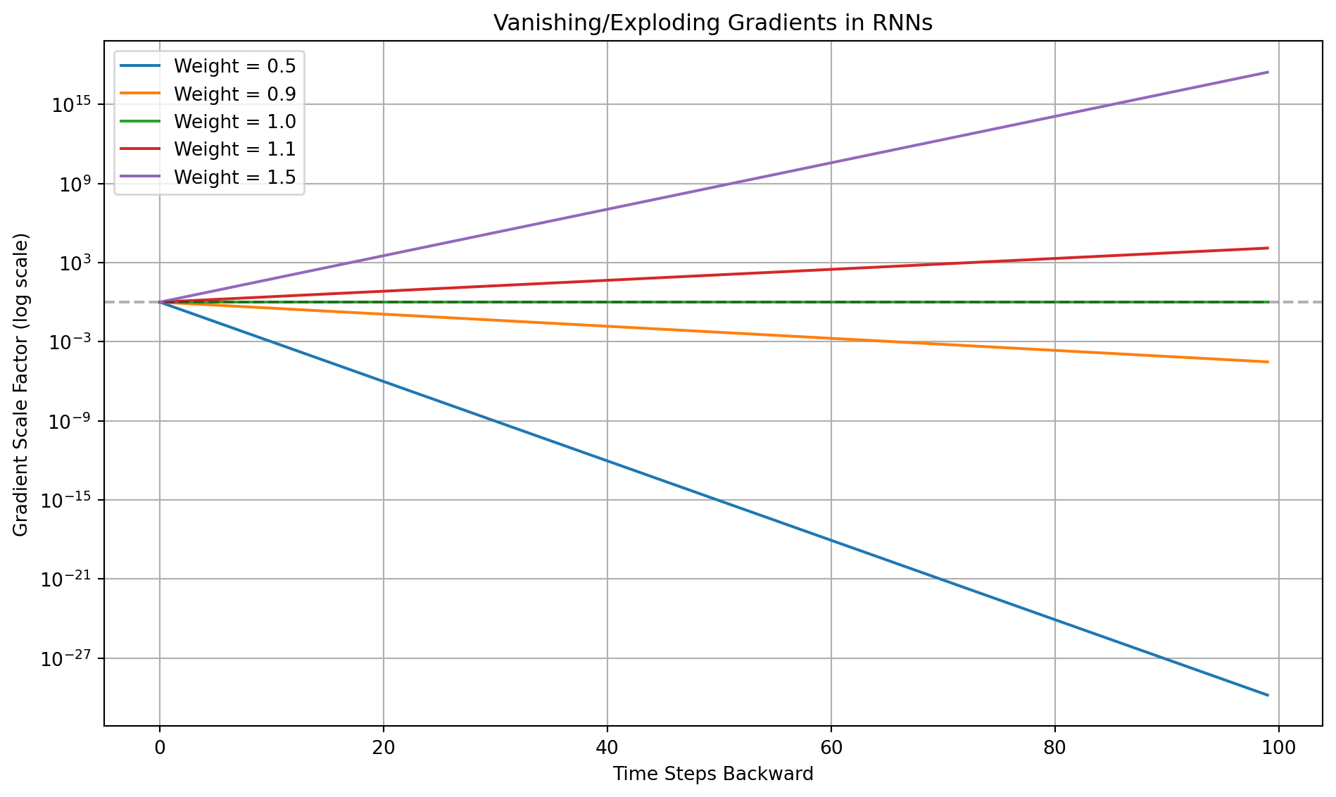
14.1.2 The Vanishing/Exploding Gradient Problem
A major challenge in training simple RNNs is the vanishing or exploding gradient problem. Because the same weight matrix is applied at each time step, backpropagation through time involves many repeated multiplications. If the recurrent weights are small, the gradient can shrink exponentially, making it impossible to learn long-range dependencies (vanishing gradient). Conversely, if the weights are large, the gradient can grow exponentially, leading to unstable training (exploding gradient).
This mathematical constraint severely limits the ability of vanilla RNNs to connect events that are far apart in a sequence, a crucial capability for understanding complex data like language or long-term patient histories.
14.1.3 LSTMs and GRUs: Gated Recurrence
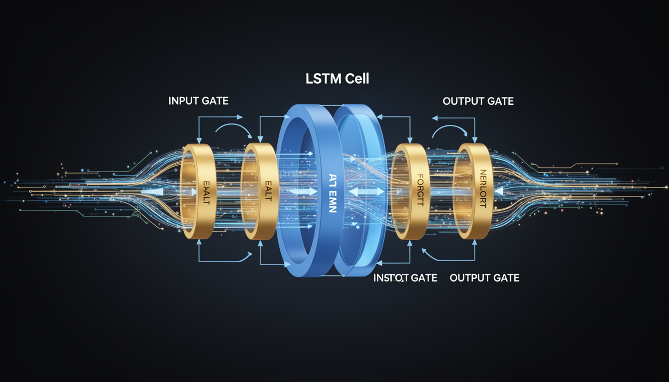
To overcome the limitations of simple RNNs, more sophisticated architectures like Long Short-Term Memory (LSTM) and Gated Recurrent Units (GRU) were developed. These models introduce gating mechanisms that allow the network to selectively add, remove, or preserve information in its memory.
LSTM Architecture
LSTMs use a dedicated cell state to carry information over long sequences, along with three gates to control this flow: 1. Forget Gate: Decides what information to discard from the cell state. 2. Input Gate: Decides which new information to store in the cell state. 3. Output Gate: Decides what information from the cell state to use for the output.
These gates act like valves, learning to open and close based on the current input and hidden state, which allows the network to maintain relevant information over long periods while ignoring irrelevant details.
GRU Architecture
GRUs are a more recent and simplified version of LSTMs. They combine the forget and input gates into a single update gate and have a reset gate that controls how much of the past information to forget. GRUs are often computationally more efficient and can perform as well as LSTMs on many tasks.
TipNeuroscience Connection: Gating in the Basal Ganglia
The gating mechanisms of LSTMs and GRUs are functionally analogous to the role of the basal ganglia in cognitive control and working memory. The basal ganglia are thought to act as a central gating system for the brain, controlling which pieces of information are allowed to enter and be maintained in the prefrontal cortex (the brain’s working memory hub).
- The Input/Update Gate resembles the basal ganglia’s function of selectively “opening the gate” to allow relevant sensory information or internal thoughts to update the contents of working memory.
- The Forget Gate is similar to mechanisms that clear or suppress outdated information from the PFC, preventing interference and allowing for flexible updates.
By learning to control information flow, these gated RNNs provide a powerful model for how the brain might dynamically manage its own memory systems.
14.1.4 Bidirectional RNNs
For many tasks, context from the future is as important as context from the past. Bidirectional RNNs address this by processing the sequence in two directions: one forward pass from start to end, and one backward pass from end to start. The outputs from both passes are then concatenated at each time step.
This allows the model to have a complete picture of the sequence when making a prediction at any given point, which is crucial for tasks like named entity recognition (e.g., knowing a word is a person’s name might depend on the words that follow it).
22.3 14.2 Attention Mechanisms
While gated RNNs improved the handling of long-range dependencies, they still struggle with extremely long sequences as they must compress the entire history into a fixed-size state vector. Attention mechanisms solve this by allowing the model to directly look at and focus on specific parts of the input sequence when producing an output, regardless of their distance.
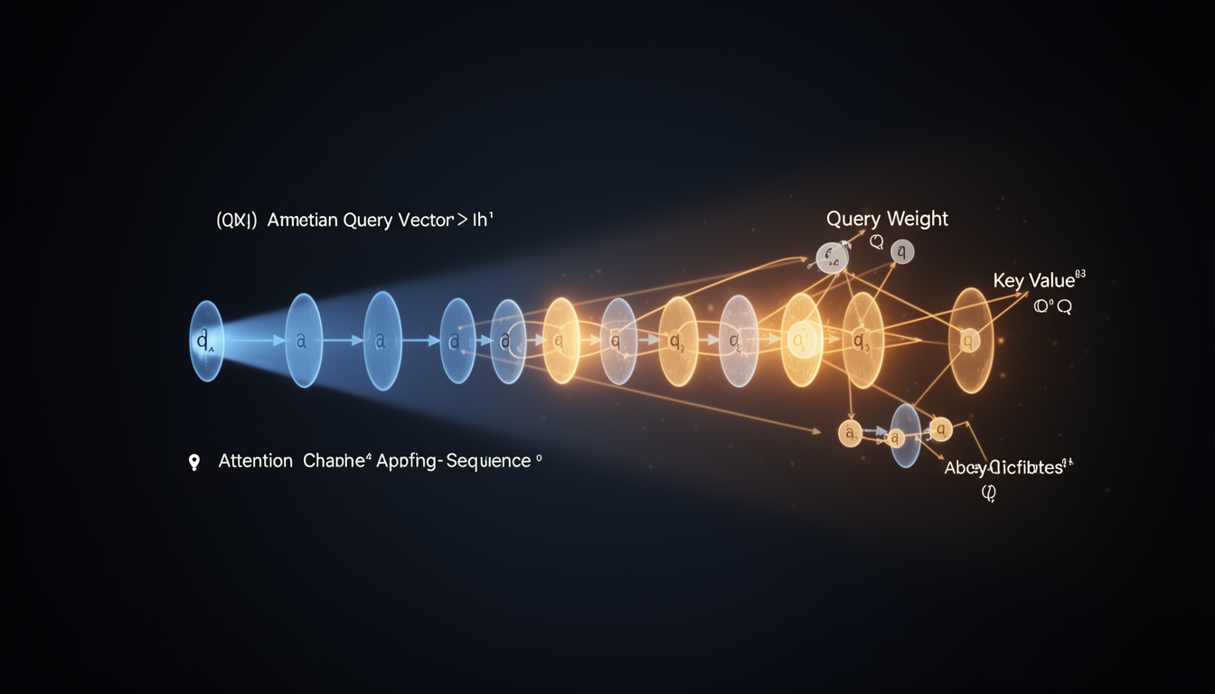
 Figure 14.2: Attention mechanism architecture showing query, key, value operations and how attention weights are computed and applied.
14.2.1 The Intuition Behind Attention
Attention was inspired by human cognition. When we translate a sentence, listen to a conversation, or describe a scene, we don’t process the entire input in one go. Instead, we focus on the most relevant parts for the task at hand. The attention mechanism formalizes this intuition. It computes a set of attention weights for each input element, indicating its relevance to the current output.
14.2.2 Self-Attention: Sequences Attending to Themselves
The key breakthrough was self-attention, where a sequence attends to itself. This allows the model to weigh the importance of all other words in the sequence when encoding a specific word. For example, when processing the word “it” in the sentence “The cat chased the mouse because it was fast,” self-attention can learn to associate “it” with “mouse.”
The mechanism works by projecting each input element into three vectors: a Query, a Key, and a Value. - The Query represents the current element’s request for information. - The Key represents what information each element has to offer. - The Value represents the content of each element.
The model computes the similarity between the Query of the current element and the Key of every other element. These similarity scores are then converted into attention weights via a softmax function, which are used to create a weighted sum of all the Values.
The self-attention operation is defined as:
\[\text{Attention}(Q, K, V) = \text{softmax}\left(\frac{QK^T}{\sqrt{d_k}}\right)V\]
14.2.3 Multi-Head Attention
Multi-Head Attention improves upon self-attention by running the mechanism multiple times in parallel with different, learned linear projections. Each “head” can learn to focus on different types of relationships (e.g., one head might track syntactic dependencies, while another tracks semantic relationships). The outputs of all heads are then concatenated and projected back to the original dimension, creating a richer representation.
TipNeuroscience Connection: Selective Attention in the Cortex
The attention mechanism in AI is a powerful abstraction of selective attention in the brain. When you focus on a particular voice in a noisy room, your brain is actively enhancing the neural representation of that voice while suppressing others. This is thought to be mediated by fronto-parietal networks that send top-down signals to sensory cortices.
- The Query is analogous to the top-down goal or context (e.g., “listen for John’s voice”).
- The Keys are like the features of all available sensory inputs (e.g., the pitch and timbre of all voices).
- The Values are the full neural representations of those inputs.
The brain computes the relevance of each input (Key) to the current goal (Query) and uses that to amplify the most relevant neural signals (Values). Multi-head attention can be seen as a parallel to the brain’s ability to attend to multiple features simultaneously (e.g., attending to both the location and color of an object).
22.4 14.3 Transformer Architecture
The Transformer, introduced in “Attention Is All You Need,” is an architecture that dispenses with recurrence entirely and relies solely on self-attention. This design choice allows for massive parallelization, enabling the training of much larger models on more data than was ever possible with RNNs.
 Figure 14.3: The Transformer architecture featuring an encoder-decoder structure with multi-head attention, positional encodings, and feed-forward networks.
The architecture consists of two main parts: 1. Encoder: A stack of layers that processes the input sequence and builds a rich, context-aware representation of it. 2. Decoder: A stack of layers that generates the output sequence one element at a time, using the encoder’s output and the previously generated elements.
Each layer in the encoder and decoder contains two main sub-layers: a multi-head self-attention mechanism and a simple, position-wise feed-forward network. Residual connections and layer normalization are used around each sub-layer to ensure stable training.
14.3.1 Positional Encodings
Since the Transformer contains no recurrence, it has no inherent sense of sequence order. To remedy this, positional encodings are added to the input embeddings. These are vectors that provide information about the position of each element in the sequence. The original paper used sine and cosine functions of different frequencies, allowing the model to easily learn to attend to relative positions.
22.5 14.4 Neural Sequence Processing
The brain is a masterful sequence processor. From understanding language to executing a motor command, neural circuits are exquisitely tuned to handle information that unfolds over time. This section bridges the artificial models we’ve discussed with their biological counterparts.
 Figure 14.4: Comparison of sequence processing mechanisms in the brain and neural networks, highlighting temporal dynamics, working memory, and hierarchical processing.
14.4.1 Temporal Dynamics in Cortical Circuits
Neural circuits exhibit rich, intrinsic dynamics that are crucial for processing sequences. Unlike feedforward networks that are silent without input, recurrent circuits in the brain can generate complex, evolving patterns of activity on their own.
- Persistent Activity: As mentioned, recurrent connections allow activity to be maintained, forming a basis for working memory.
- Sequential Activation: Specific connectivity patterns can cause “waves” of neural activity to propagate through a network, creating an internal clock or sequence generator. This is observed in brain regions like the hippocampus during memory recall and the motor cortex during movement execution.
- Temporal Integration: Neurons act as integrators, summing inputs over time. Different neuron types have different time constants, allowing the brain to process information across multiple timescales simultaneously.
Connection to AI Models: The hidden state of an RNN is a direct, albeit simplified, model of these population dynamics. The learned recurrent weights (\(W_{hh}\)) define the rules by which the neural state evolves, attempting to capture the complex temporal patterns inherent in the data.
14.4.2 Predictive Processing
A leading theory in neuroscience, predictive coding, posits that the brain is a prediction machine. It constantly generates top-down predictions about upcoming sensory input and uses bottom-up sensory signals to compute prediction errors—the mismatch between expectation and reality. These errors are then used to update the brain’s internal model of the world.
- Hierarchical Predictions: This process is hierarchical. Higher brain areas (like the prefrontal cortex) generate abstract predictions (e.g., “I’m about to see a face”), which are translated into more concrete predictions by lower sensory areas (e.g., “I expect to see an oval shape with two horizontally aligned dots”).
- Error Signaling: Only the error signals are propagated up the hierarchy, making for an extremely efficient coding scheme.
Connection to AI Models: This is remarkably similar to how modern language models are trained. Models like GPT are trained on a simple objective: predict the next word in a sequence. They are, in essence, predictive coding machines. The loss function in training is a measure of prediction error, which drives the learning process, refining the model’s internal representation of language.
14.4.3 Hierarchical Temporal Processing
The brain processes sequences across a hierarchy of timescales. - Primary auditory cortex responds to rapid changes in sound (milliseconds). - Secondary auditory cortex integrates sounds into phonemes and words (tens to hundreds of milliseconds). - Broca’s and Wernicke’s areas process syntax and semantics over seconds. - The hippocampus and prefrontal cortex can link events over many minutes or even hours.
Connection to AI Models: Stacked RNNs or Transformers create a similar hierarchy. Lower layers in a Transformer tend to learn local, syntactic relationships, while higher layers learn to integrate information over longer distances to capture more abstract, semantic, and contextual meaning. The multi-head attention mechanism allows different heads to specialize in different temporal scales and relationship types, mirroring the functional specialization of different brain areas.
22.6 14.5 Applications in Healthcare and Neuroscience
Sequence models are not just for language; they are powerful tools for analyzing any form of sequential data, including the complex time-series data found in healthcare and neuroscience.
14.5.1 Modeling Neural Data
RNNs and Transformers can be trained on time-series data from neural recordings (e.g., EEG, MEG, or multi-unit recordings) to model the dynamics of neural circuits. By training a model to predict future neural activity from past activity, researchers can develop an in silico model of a brain region. This model can then be analyzed to understand how the circuit processes information, generates patterns, or even how it might be affected by disease or drugs.
14.5.2 Clinical Applications: Healthcare Time Series
Electronic Health Records (EHR) are inherently sequential. A patient’s journey is a sequence of diagnoses, medications, lab tests, and procedures over time. Sequence models are uniquely suited to analyze this data.
- Disease Progression Modeling: An LSTM or Transformer can be trained on the records of thousands of patients to learn the typical progression of a disease like diabetes or heart failure. This can be used to predict a new patient’s future risk of complications.
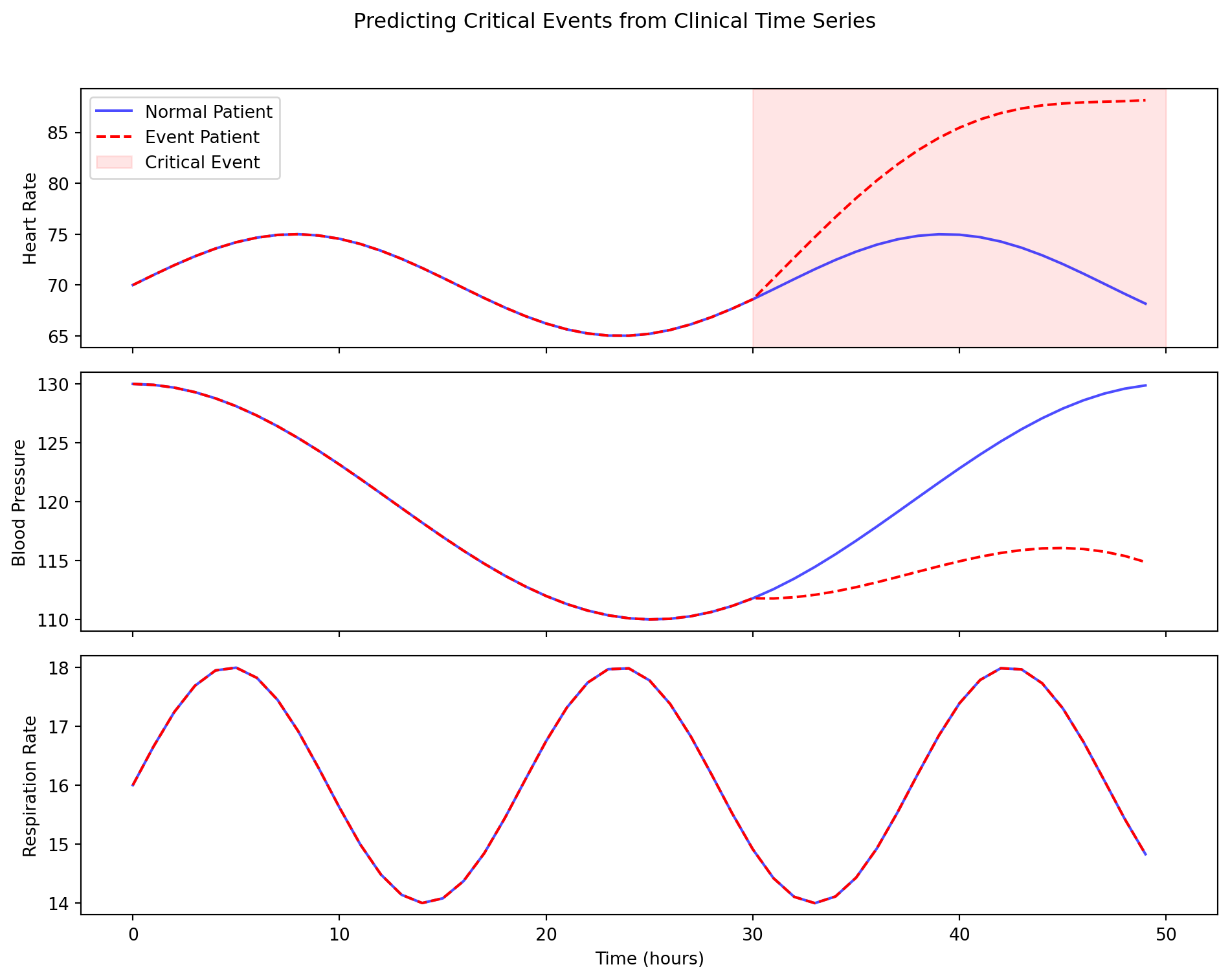
- Predictive Alerts: Models can monitor real-time data from ICU patients (heart rate, blood pressure, etc.) to predict the onset of critical events like sepsis or cardiac arrest hours before they would be apparent to a human clinician.
- Treatment Recommendation: By analyzing the treatment sequences of past patients and their outcomes, models can suggest the next best medication or intervention for a current patient.
A key challenge in this domain is that clinical data is often irregularly sampled (e.g., a patient has lab tests done weeks apart, then several in one day) and contains missing values. Modern architectures, often based on attention, are being developed to specifically handle these challenges by learning to model the time gaps and impute missing information.

ImportantChapter Summary
In this chapter, we journeyed from the fundamentals of text processing through the evolution of sequence models, culminating in the state-of-the-art Transformer architecture.
- Text Processing Fundamentals showed how continuous signals (speech or unsegmented text) must be discretized into tokens, a challenge the brain solves through statistical learning, and computers solve through tokenization algorithms.
- Classical Preprocessing including stemming, lemmatization, and TF-IDF vectorization prepared the ground for neural approaches by establishing how to normalize and represent text numerically.
- Recurrent Neural Networks (RNNs) introduced the idea of a hidden state to maintain memory of past information, but were limited by the vanishing gradient problem.
- LSTMs and GRUs solved this with gating mechanisms, enabling the learning of much longer-term dependencies and drawing parallels to gating in the brain’s basal ganglia.
- Attention Mechanisms provided a new paradigm, allowing models to dynamically focus on the most relevant parts of the input sequence, similar to selective attention in the cortex.
- The Transformer architecture abandoned recurrence entirely, relying solely on self-attention. This enabled massive parallelization and has become the foundation for most modern large-scale models.
- We explored the deep connections to neuroscience, seeing how RNNs model persistent activity, gates mimic the basal ganglia, attention reflects cortical selective attention, and the predictive nature of Transformers aligns with the theory of the brain as a prediction machine.
- Finally, we saw how these models are applied to clinical time-series data, offering powerful new ways to predict disease progression and improve patient care.
ImportantKnowledge Connections
Looking Back - Chapter 10 (Deep Learning): The optimization techniques and architectural principles from the previous chapter are the building blocks for all the sequence models discussed here.
Looking Forward - Chapter 12 (Large Language Models): The Transformer architecture is the absolute foundation for the Large Language Models (LLMs) we will explore in the next chapter. - Chapter 17 (BCIs): Sequence models are critical for decoding neural signals (which are time-series data) in Brain-Computer Interfaces.
22.7 Exercises
Conceptual Questions
Gating Mechanisms and the Basal Ganglia: Explain how the gating mechanisms in LSTMs (forget gate, input gate, output gate) conceptually parallel the role of the basal ganglia in working memory. What computational problem do both systems solve, and why is selective gating necessary for effective sequence processing?
Attention vs. Recurrence: Compare and contrast how RNNs and attention mechanisms handle long-range dependencies in sequences. Why did the Transformer architecture choose to completely abandon recurrence in favor of pure attention? What are the computational and representational tradeoffs of this choice?
Positional Encodings: The Transformer has no inherent notion of sequence order, requiring explicit positional encodings. In contrast, RNNs inherently encode position through their sequential processing. Discuss the advantages and disadvantages of each approach. How might the brain encode temporal order in neural sequences?
Predictive Processing in Language: The chapter connects LLM training (next-word prediction) to the predictive processing framework in neuroscience. Explain this connection in detail. What neural signals in the brain might correspond to “prediction errors” when processing language? How does this relate to phenomena like the N400 ERP component?
Computational Problems
- Building a Character-Level RNN: Implement a character-level RNN for text generation from scratch using PyTorch or TensorFlow. Train it on a small corpus (e.g., Shakespeare, code, or scientific abstracts). Your implementation should:
- Use an LSTM or GRU cell
- Implement teacher forcing during training
- Generate new text by sampling from the model
- Visualize the hidden state activations over time for a sample sequence
- Analyze what linguistic patterns the model has learned at different layers
- Attention Visualization: Implement a simple self-attention mechanism and visualize the attention weights for a sample sentence. Specifically:
- Compute Query, Key, and Value matrices for each word
- Calculate attention scores and apply softmax
- Create a heatmap showing which words attend to which other words
- Experiment with multi-head attention and show how different heads learn to attend to different patterns (e.g., syntactic vs. semantic relationships)
- Vanishing Gradient Analysis: Empirically demonstrate the vanishing gradient problem in vanilla RNNs:
- Create a simple copy task where the model must remember and reproduce a sequence after a variable delay
- Train vanilla RNNs with different sequence lengths (10, 50, 100, 200 steps)
- Plot gradient magnitudes as they backpropagate through time
- Repeat with an LSTM and compare the gradient flow
- Determine the maximum sequence length each architecture can reliably learn
- Clinical Time-Series Prediction: Using a publicly available medical dataset (e.g., MIMIC-III or PhysioNet), build a sequence model to predict a clinical outcome:
- Handle irregular sampling and missing data
- Implement a Transformer or LSTM-based model with time-aware encodings
- Compare performance with and without attention mechanisms
- Interpret what temporal patterns the model has learned (e.g., using attention weights)
Discussion Questions
Transformers and Biological Plausibility: While Transformers are highly effective, the self-attention mechanism requires each element to simultaneously “see” all other elements in the sequence, which is not biologically plausible (the brain processes information in real-time without looking into the future). Discuss potential modifications to the Transformer architecture that would make it more aligned with how the brain processes sequences. Are there recent architecture proposals that attempt to bridge this gap?
Sequence Models in Neuroscience Research: Propose three specific research questions in neuroscience where sequence models would be particularly valuable. For each:
- Describe the sequential data you would analyze (e.g., spike trains, fMRI time series, behavioral trajectories)
- Specify which architecture (RNN, LSTM, Transformer) would be most appropriate and why
- Explain what scientific insights you hope to gain from the model’s learned representations or predictions
- Discuss potential limitations or confounds in interpreting the model’s behavior as a model of brain function
22.8 References
Bahdanau, D., Cho, K., & Bengio, Y. (2015). Neural machine translation by jointly learning to align and translate. International Conference on Learning Representations. https://arxiv.org/abs/1409.0473
Bengio, Y., Simard, P., & Frasconi, P. (1994). Learning long-term dependencies with gradient descent is difficult. IEEE Transactions on Neural Networks, 5(2), 157-166. https://doi.org/10.1109/72.279181
Cho, K., van Merriënboer, B., Gulcehre, C., Bahdanau, D., Bougares, F., Schwenk, H., & Bengio, Y. (2014). Learning phrase representations using RNN encoder-decoder for statistical machine translation. Conference on Empirical Methods in Natural Language Processing. https://arxiv.org/abs/1406.1078
Chung, J., Gulcehre, C., Cho, K., & Bengio, Y. (2014). Empirical evaluation of gated recurrent neural networks on sequence modeling. NIPS 2014 Workshop on Deep Learning. https://arxiv.org/abs/1412.3555
Elman, J. L. (1990). Finding structure in time. Cognitive Science, 14(2), 179-211. https://doi.org/10.1207/s15516709cog1402_1
Graves, A. (2013). Generating sequences with recurrent neural networks. arXiv preprint arXiv:1308.0850. https://arxiv.org/abs/1308.0850
Hochreiter, S., & Schmidhuber, J. (1997). Long short-term memory. Neural Computation, 9(8), 1735-1780. https://doi.org/10.1162/neco.1997.9.8.1735
Luong, M. T., Pham, H., & Manning, C. D. (2015). Effective approaches to attention-based neural machine translation. Conference on Empirical Methods in Natural Language Processing. https://arxiv.org/abs/1508.04025
O’Keefe, J., & Dostrovsky, J. (1971). The hippocampus as a spatial map: Preliminary evidence from unit activity in the freely-moving rat. Brain Research, 34(1), 171-175.
Pascanu, R., Mikolov, T., & Bengio, Y. (2013). On the difficulty of training recurrent neural networks. International Conference on Machine Learning. https://arxiv.org/abs/1211.5063
Schuster, M., & Paliwal, K. K. (1997). Bidirectional recurrent neural networks. IEEE Transactions on Signal Processing, 45(11), 2673-2681. https://doi.org/10.1109/78.650093
Vaswani, A., Shazeer, N., Parmar, N., Uszkoreit, J., Jones, L., Gomez, A. N., Kaiser, Ł., & Polosukhin, I. (2017). Attention is all you need. Advances in Neural Information Processing Systems, 30. https://arxiv.org/abs/1706.03762