23 Large Language Models & Fine-Tuning
NoteLearning Objectives
By the end of this chapter, you will be able to:
- Understand large language model architectures and pretraining strategies
- Master subword tokenization algorithms (BPE, WordPiece) and their connection to morphology
- Master fine-tuning techniques and parameter-efficient adaptation methods
- Connect computational language models to human language processing mechanisms
- Implement effective prompting strategies and model adaptations
- Apply quantization and model optimization techniques for efficient deployment
- Evaluate LLM performance and understand its critical limitations
23.1 15.1 Large Language Model Fundamentals

Large Language Models (LLMs) represent a paradigm shift in artificial intelligence. They are not merely larger versions of previous models; their scale has unlocked qualitatively new abilities, moving AI from narrow specialists to general-purpose reasoning engines. This section explores the foundational elements that make these powerful models possible.
NoteWhy LLMs Changed Everything
Before LLMs, AI systems were typically narrow specialists—a model for chess, another for image classification, a third for speech recognition. LLMs shattered this paradigm by demonstrating that a single, massive model trained on a simple objective—predicting the next word—could acquire a vast range of skills without being explicitly taught them.
This is a phase transition. Like water becoming steam, sufficiently large language models exhibit emergent abilities: - In-context learning: Learning a new task from just a few examples in a prompt. - Chain-of-thought reasoning: Solving a problem by “thinking out loud” in steps. - Instruction following: Executing complex commands given in natural language.
Understanding how these capabilities arise from a simple predictive objective is one of the deepest and most active areas of research in modern AI.
 Figure 15.1: Large Language Model architecture, showing the progression from input tokenization through transformer layers to next token prediction.

15.1.1 Transformer-Based Architectures
Modern LLMs are almost exclusively built on the Transformer architecture (Chapter 11). While the core components are the same, LLMs leverage several key modifications and, most importantly, unprecedented scale.
Key architectural features include: 1. Scale: Modern LLMs have billions or even trillions of parameters, compared to the hundreds of millions in earlier models. This sheer scale is the primary driver of their advanced capabilities. 2. Decoder-Only Architecture: Many of the most successful LLMs (like the GPT series) are “decoder-only” models. They discard the encoder part of the original Transformer and use a stack of decoder layers, making them highly effective at generating coherent text based on a prompt. 3. Architectural Refinements: Minor but important tweaks are common, such as using pre-normalization, different activation functions (like GELU or SwiGLU), and more efficient attention mechanisms (like Flash Attention) to handle longer sequences.
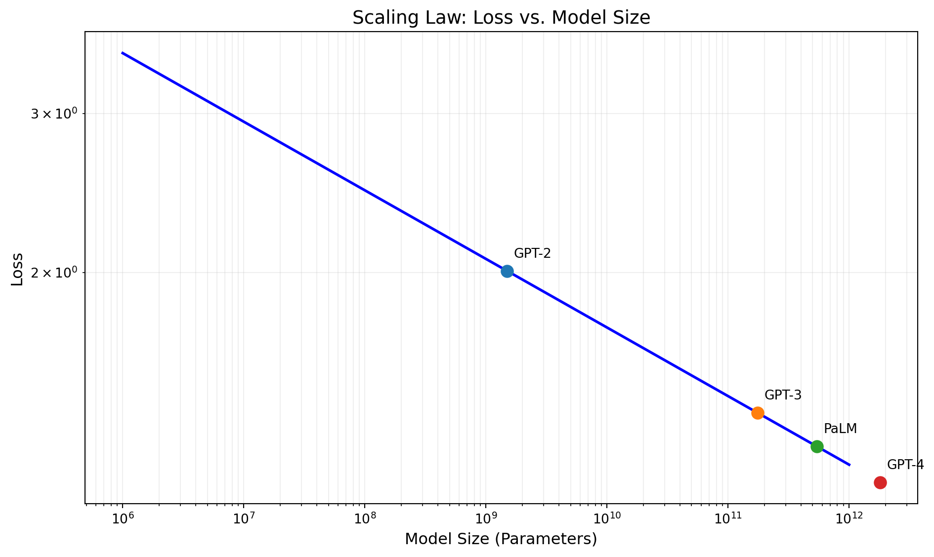
15.1.2 Scaling Laws and Emergent Abilities
The discovery of scaling laws was a pivotal moment in AI. Researchers found that an LLM’s performance improves predictably as a power-law function of three factors: the number of model parameters, the size of the training dataset, and the amount of compute used for training.
ImportantThe Magic of Scale
The scaling laws provided a recipe for creating more powerful AI: simply make everything bigger. This led to what AI researcher Rich Sutton called “The Bitter Lesson”: methods that leverage computation and scale have consistently outperformed those that rely on intricate, human-designed features.
- Predictable Improvement: The power-law relationship means you can accurately predict how much better a model will be if you increase its size or training data by 10x. This turned AI research from a series of unpredictable breakthroughs into a more systematic engineering discipline.
- Emergent Abilities: The most fascinating outcome of scale is the emergence of abilities that are absent in smaller models. Capabilities like arithmetic, multi-step reasoning, and instruction following don’t improve gradually; they appear to “switch on” once a model crosses a certain size threshold. This suggests that quantitative increases in scale can lead to qualitative leaps in intelligence.
15.1.3 From Text to Tokens: Subword Tokenization
Before text can enter a neural network, it must be converted into a sequence of discrete units. The choice of these units (characters, words, or something in between) profoundly affects model performance. Modern LLMs have converged on subword tokenization, a technique that elegantly balances vocabulary size against sequence length.
The Vocabulary Trade-off
Consider the extremes:
- Character-level: Every letter is a token. Vocabulary is tiny (~100 symbols), but sequences become very long (“artificial intelligence” = 23 tokens), making attention expensive and long-range dependencies harder to learn.
- Word-level: Every word is a token. Sequences are short, but vocabulary explodes. With millions of possible words (including proper nouns, technical terms, and misspellings), most words appear rarely, and novel words are impossible to represent.
Subword tokenization finds the sweet spot: common words like “the” remain single tokens, while rare words like “tokenization” are split into meaningful pieces (“token” + “ization”). This keeps vocabulary manageable (typically 32,000–100,000 tokens) while handling any input.
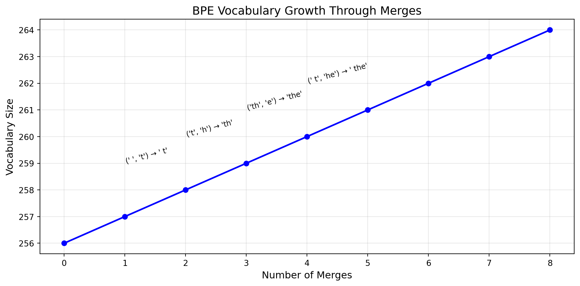
Byte-Pair Encoding (BPE)
BPE, originally a data compression algorithm, became the dominant tokenization method for LLMs after its adaptation for NLP.
The Algorithm:
- Initialize: Start with a vocabulary of all individual characters (or bytes) in the training corpus
- Count pairs: Find the most frequently occurring adjacent pair of tokens
- Merge: Create a new token by combining this pair; add it to the vocabulary
- Repeat: Continue until the vocabulary reaches the desired size
Example: Starting with the word “lowest” and a character vocabulary:
Iteration 0: ['l', 'o', 'w', 'e', 's', 't']
Most frequent pair: ('e', 's') → merge to 'es'
Iteration 1: ['l', 'o', 'w', 'es', 't']
Most frequent pair: ('es', 't') → merge to 'est'
Iteration 2: ['l', 'o', 'w', 'est']
Most frequent pair: ('l', 'o') → merge to 'lo'
Iteration 3: ['lo', 'w', 'est']
...
After training on a large corpus, BPE learns meaningful subword units: - Common morphemes: “un-”, “-ing”, “-tion”, “-est” - Frequent words as single tokens: “the”, “and”, “is” - Rare words split sensibly: “cryptocurrency” → [“crypt”, “o”, “currency”]
Key Properties: - Deterministic: Same vocabulary always produces the same tokenization - Open vocabulary: Any text can be tokenized, even with novel words - Frequency-adaptive: Common patterns become single tokens
WordPiece and SentencePiece
WordPiece (used by BERT) is similar to BPE but selects merges based on likelihood improvement rather than raw frequency. It uses a “##” prefix to mark subword continuations: “tokenization” → [“token”, “##ization”].
SentencePiece treats the input as a raw byte stream, making it language-agnostic and able to handle any script without language-specific preprocessing. It can implement either BPE or a unigram language model approach. GPT models use a variant called Byte-level BPE that operates on UTF-8 bytes.
TipNeuroscience Connection: Morphological Decomposition in the Brain
The subword units learned by BPE often correspond to morphemes, the smallest meaning-bearing units in language. This is not coincidental. The training objective (maximizing compression / minimizing tokens) naturally discovers linguistic structure.
The brain similarly decomposes words into morphological units during reading: - Visual Word Form Area: Initial processing of the full word - Left Inferior Frontal Gyrus: Decomposition into stems and affixes - Priming effects: Seeing “walked” speeds recognition of “walk,” suggesting automatic decomposition
Neuroimaging studies show that morphologically complex words (“unhappiness”) activate different patterns than simple words, with additional processing in Broca’s area for combining morpheme meanings. BPE’s learned vocabulary can be seen as an approximation to the brain’s morphological lexicon, a compressed representation that balances storage efficiency with compositional expressivity.
Why Tokenization Matters
Tokenization choices have surprising downstream effects:
Arithmetic: GPT-3 struggles with multi-digit arithmetic partly because numbers are tokenized inconsistently. “380” might be one token while “381” is two (“38” + “1”), making pattern recognition difficult.
Multilingual Performance: BPE trained primarily on English tends to over-segment other languages, making non-English text 2-4x longer in tokens and proportionally harder to process within fixed context windows.
Prompt Length: Every token counts against the context window. Understanding tokenization helps craft efficient prompts.
Novel Words: Words not seen during BPE training (like new technical terms) may be inefficiently split, affecting model performance on specialized domains.

15.1.4 Pre-training Objectives
LLMs are trained using self-supervised learning on vast corpora of text and code. The most common objective is next-token prediction (also called causal language modeling). The model is given a sequence of text and its only task is to predict the very next word or sub-word token.
By performing this simple task billions of times on a dataset spanning a significant fraction of the internet, the model is forced to learn grammar, facts, reasoning abilities, and a sophisticated internal representation of the world to make its predictions as accurate as possible.
TipNeuroscience Connection: Predictive Processing
The training objective of LLMs is remarkably consistent with the predictive processing framework in neuroscience. This theory posits that the brain is fundamentally a prediction machine, constantly generating top-down predictions about upcoming sensory input. When a mismatch occurs (a “prediction error”), the brain updates its internal models.
- LLM Training: The model predicts the next token, compares its prediction to the actual token, and uses the error (loss) to update its weights via backpropagation.
- Brain Learning: The brain predicts the next word in a sentence. If it hears an unexpected word, it generates a specific neural signal (like the N400 event-related potential) that is thought to reflect this prediction error and drive synaptic plasticity.
Both systems learn rich world models by minimizing prediction error, suggesting a deep, convergent principle for learning in both biological and artificial neural networks.
15.1.5 Encoder Models: BERT and Bidirectional Understanding
While GPT-style models generate text left-to-right, another family of models (the encoder-only Transformers) takes a fundamentally different approach. The most famous is BERT (Bidirectional Encoder Representations from Transformers), which revolutionized NLP in 2018.
Autoregressive vs. Bidirectional
The key distinction:
Autoregressive (GPT): Each token can only attend to tokens before it. This enables generation but limits understanding. When processing “The mouse ran from the cat,” GPT encodes “mouse” without knowing a cat is coming.
Bidirectional (BERT): Each token can attend to tokens in both directions. When encoding “mouse,” BERT sees the entire sentence, understanding from context that this is prey, not a computer peripheral.
This bidirectional context is powerful for understanding tasks (classification, question answering, named entity recognition) but makes generation difficult. You can’t predict the next word if you’re already looking at it.
Masked Language Modeling (MLM)
BERT is trained using masked language modeling: randomly mask 15% of input tokens and train the model to predict the original words from context.
For example: - Input: “The [MASK] sat on the [MASK]” - Target: Predict “cat” and “mat”
This forces the model to build deep bidirectional representations. Understanding that “[MASK] sat on the” probably refers to an animal requires integrating context from both sides.
The masking strategy is carefully designed: - 80% of masked positions: Replace with [MASK] token - 10%: Replace with random word - 10%: Keep original word
This prevents the model from only learning to predict [MASK] tokens.
BERT vs. GPT: Complementary Strengths
| Aspect | BERT (Encoder) | GPT (Decoder) |
|---|---|---|
| Attention | Bidirectional | Causal (left-to-right) |
| Training | Masked LM + Next Sentence | Next token prediction |
| Best for | Understanding, classification | Generation, dialogue |
| Context | Full sentence at once | Sequential processing |
BERT variants: - RoBERTa: Better training (more data, no next-sentence prediction) - DistilBERT: 40% smaller, 60% faster, 97% of performance - ALBERT: Parameter sharing for efficiency - XLNet: Permutation-based training combining benefits of both
TipNeuroscience Connection: Feedforward vs. Recurrent Processing in Visual Cortex
The encoder/decoder distinction in Transformers parallels two modes of processing in the brain:
Feedforward processing (like GPT’s causal attention): Information flows in one direction through the visual hierarchy. Fast (~100ms) but limited. You can recognize an object before fully understanding the scene.
Recurrent processing (like BERT’s bidirectional attention): Information flows back and forth, allowing context from “later” areas to influence “earlier” representations. Slower but enables contextual integration. You understand that a blob is a cat because it’s being chased by a dog.
Studies using backward masking (briefly showing an image, then disrupting it) demonstrate that complex scene understanding requires recurrent processing, just as BERT’s bidirectional attention enables deeper language understanding than purely feedforward models.
Contextual Embeddings: Words in Context
Unlike Word2Vec (one vector per word), BERT produces contextual embeddings, meaning different vectors for the same word in different contexts:
- “I went to the bank to deposit money” → financial institution
- “I sat on the river bank” → riverside
The embedding for “bank” differs in each sentence because BERT’s attention mechanism integrates the surrounding context. This is a major advance over static embeddings and closely parallels how the brain processes word meaning through context-dependent activation in semantic areas like the angular gyrus.
23.2 15.2 Fine-tuning Methods
While pre-training endows LLMs with general knowledge, fine-tuning adapts them to specific tasks or domains. This process involves continuing the training on a smaller, curated dataset.
NoteThe Fine-Tuning Paradox
Here’s the paradox: LLMs seem to know almost everything but often fail at specific, simple tasks out of the box. It’s like a brilliant professor who can discuss quantum physics but can’t follow your company’s email formatting rules. Fine-tuning is less about teaching the model new knowledge and more about teaching it new behaviors.
- Pre-training is for learning what to know (facts, language, reasoning).
- Fine-tuning is for learning how to behave (style, format, constraints).
- RLHF (discussed later) is for learning what humans prefer (helpfulness, safety).
The challenge is that fine-tuning a trillion-parameter model is immensely expensive. This has led to an explosion of research into parameter-efficient methods that can achieve similar results by updating less than 1% of the model’s weights.
 Figure 15.2: Comparison of LLM fine-tuning methods, from resource-intensive full fine-tuning to parameter-efficient techniques like LoRA and RLHF.
15.2.1 Full Fine-tuning
This is the most straightforward approach: update all the weights of the pre-trained model on the new dataset. While it often yields the best performance, it is computationally intensive and requires storing a full new copy of the model for each task. A major risk is catastrophic forgetting, where the model loses some of its general capabilities by overfitting to the narrow fine-tuning dataset.
15.2.2 Parameter-Efficient Fine-Tuning (PEFT)
PEFT methods dramatically reduce the cost of fine-tuning by freezing the vast majority of the pre-trained model’s parameters and only updating a small, targeted subset.
NoteThe College vs. On-the-Job Training Analogy
Imagine a high school graduate entering the workforce. There are fundamentally different ways to develop their skills:
Full Fine-tuning = College (4-5 Years)
Sending someone to college is expensive and time-consuming, but transformative. They read hundreds of books, attend thousands of lectures, and write countless papers. Over four to five years, this intensive learning literally rewires their neurons. They emerge as a different person with deeply integrated knowledge. This is full fine-tuning: you put the model through extensive additional training, updating billions of weights. The model’s entire neural network is modified to incorporate the new knowledge. It’s powerful but computationally expensive, and you need to be careful not to overwrite what the model already knew.
LoRA = On-the-Job Training with a Script
Now imagine instead you hire that same high school graduate and hand them a script: “When a customer asks about returns, say this. When they ask about hours, say that.” You haven’t changed who they fundamentally are. Their education, personality, and general knowledge remain untouched. You’ve just given them a small set of specific responses for specific situations. This is LoRA (Low-Rank Adaptation): you freeze the entire pre-trained model (their brain stays as-is) and train only a tiny adapter (the script) that modifies outputs in targeted ways.
The script doesn’t require years of education. It’s learned in days and takes almost no storage. But for the specific job, it’s remarkably effective. The employee knows exactly what to say when, and that’s often all you need.
| Approach | Analogy | Trainable Parameters | Training Cost | Storage |
|---|---|---|---|---|
| Full Fine-tuning | 4 years of college | 100% (all weights) | Very high | Full model copy |
| LoRA | On-the-job script | ~0.1% (adapter only) | Low | Small adapter file |
| Prompt Tuning | Giving hints before a test | ~0.01% | Very low | Tiny prompt |
LoRA (Low-Rank Adaptation) is the most popular PEFT technique. Instead of updating the large weight matrices of the model directly, LoRA inserts small, trainable “adapter” matrices alongside them. The original weights remain frozen, and only the new, low-rank matrices are trained.
How LoRA Works Mathematically
In a standard Transformer, attention layers use weight matrices like \(W_q\), \(W_k\), \(W_v\) with dimensions \(d \times d\) (often 4096 × 4096 for large models). Fine-tuning would update all ~16 million parameters in each matrix.
LoRA instead learns a low-rank decomposition of the weight update:
\[\Delta W = BA\]
where: - \(B\) has dimensions \(d \times r\) (e.g., 4096 × 8) - \(A\) has dimensions \(r \times d\) (e.g., 8 × 4096) - \(r\) is the rank (typically 4-64, much smaller than \(d\))
The effective weight becomes \(W' = W + BA\), but we only train \(B\) and \(A\).
Parameter Reduction: - Original \(W\): \(d \times d = 16,777,216\) parameters - LoRA with \(r=8\): \((d \times r) + (r \times d) = 65,536\) parameters - Reduction: 256× (99.6% fewer trainable parameters)
During inference, you can either: 1. Keep adapters separate (easily swap between different fine-tunes) 2. Merge: \(W' = W + BA\) (no latency overhead, permanent change)
Practical LoRA Usage
# Example: Loading a base model with a LoRA adapter
from peft import PeftModel
from transformers import AutoModelForCausalLM

# Load base model (frozen)
base_model = AutoModelForCausalLM.from_pretrained("meta-llama/Llama-2-7b-hf")

# Load LoRA adapter (tiny, task-specific)
model = PeftModel.from_pretrained(base_model, "username/my-lora-adapter")
# The adapter might be only 10-50MB for a 14GB base model!
Common LoRA Configurations:
| Use Case | Rank (r) | Target Modules | Trainable Params |
|---|---|---|---|
| Light customization | 4-8 | q_proj, v_proj | ~0.05% |
| General fine-tuning | 16-32 | q, k, v, o_proj | ~0.2% |
| Complex adaptation | 64-128 | All linear layers | ~1% |
Other PEFT Techniques:
Adapter Layers: Inserting small, trainable feed-forward networks between the existing layers of the model. Like giving the employee a “decision flowchart” that they consult between steps.
Prompt Tuning: Keeping the model entirely frozen and only training a “soft prompt,” which is a sequence of trainable vectors prepended to the input. Like whispering a hint to the employee before each customer interaction.
QLoRA: Combines quantization (INT4) with LoRA, enabling fine-tuning of 65B models on a single GPU.
TipNeuroscience Connection: Task-Specific Subnetworks
PEFT methods are analogous to how the brain learns new skills without overwriting existing ones. When you learn to play tennis, you don’t rewire your entire motor cortex. Instead, your brain is thought to refine and strengthen a specific subnetwork of neurons relevant to the new skill.
- The frozen pre-trained model is like the brain’s vast, stable knowledge base and existing neural pathways.
- The PEFT adapter (like LoRA) is like the small, plastic subnetwork that is rapidly modified to encode the new skill.
The Complementary Learning Systems Theory: The brain may implement something similar to LoRA through its two memory systems: - Neocortex: Slow-learning, stores generalized knowledge (like the frozen base model) - Hippocampus: Fast-learning, handles specific episodes (like the LoRA adapter)
New information is first encoded rapidly in the hippocampus, then gradually consolidated into the neocortex during sleep. This is a biological version of training an adapter, then optionally merging it into the base model.
This approach allows for efficient and modular learning, where new abilities can be “plugged in” without disrupting the entire system, mirroring the brain’s remarkable ability to learn continuously throughout life.
15.2.3 Instruction Fine-tuning and RLHF
Modern chatbots are not just pre-trained; they undergo extensive alignment tuning to make them helpful, harmless, and honest. This is a multi-stage process:
- Instruction Fine-tuning: The model is first fine-tuned on a dataset of high-quality instruction-response pairs (e.g., “Question: What is the capital of France? Answer: The capital of France is Paris.”). This teaches the model to follow instructions and adopt a helpful conversational style.
- Reinforcement Learning from Human Feedback (RLHF): To refine the model’s behavior further, a reward model is trained on human preference data. Human labelers are shown two different responses to the same prompt and asked to choose which one is better. The reward model learns to predict which response a human would prefer. Finally, the LLM is fine-tuned using reinforcement learning (specifically, PPO) to maximize the score it receives from this reward model. This process steers the model towards outputs that are more aligned with human values.
23.3 15.3 Prompting Techniques
Prompt engineering is the art and science of designing inputs to elicit desired behaviors from an LLM without updating its weights.
 Figure 15.3: Various prompting techniques for LLMs, from zero-shot to chain-of-thought prompting and system prompt design.
15.3.1 Zero-Shot and Few-Shot Prompting
- Zero-Shot: Simply asking the model to perform a task directly. (e.g., “Translate this to French: …”)
- Few-Shot: Providing a few examples of the task in the prompt to show the model the desired input-output pattern. This leverages the model’s in-context learning ability.
15.3.2 Chain-of-Thought (CoT) Prompting
For complex reasoning tasks, LLMs often fail if asked to produce the answer directly. Chain-of-Thought prompting encourages the model to “think step by step.” By providing examples in the prompt that include a reasoning process, or by simply adding the phrase “Let’s think step by step,” the model is guided to break down the problem, which dramatically improves its performance on arithmetic, commonsense, and symbolic reasoning tasks.
TipNeuroscience Connection: Explicit vs. Implicit Reasoning
The difference between standard and CoT prompting mirrors the distinction between two modes of human thought, often called System 1 (fast, intuitive, implicit) and System 2 (slow, deliberate, explicit).
- Standard Prompting is like asking for a System 1 response. The model provides a quick, intuitive answer based on pattern matching.
- Chain-of-Thought Prompting engages a process analogous to System 2. It forces the model to slow down, externalize its reasoning process, and follow a logical sequence.
Just as humans are more likely to solve a complex problem by writing down the steps, LLMs benefit from articulating their “thought process.” This suggests that the internal monologue or step-by-step reasoning is not just a human quirk but a fundamental strategy for robust problem-solving in complex systems.
23.4 15.4 Neural Basis of Language
While LLMs are not models of the brain, their success has sparked renewed interest in comparing their mechanisms to what is known about human language processing.
 Figure 15.4: Key language processing areas in the human brain and their functional parallels in large language models.
15.4.1 Language Areas in the Brain
The human brain has a network of specialized regions for language: - Broca’s Area (inferior frontal gyrus) is crucial for syntax and speech production. Damage here leads to difficulty forming grammatically correct sentences. - Wernicke’s Area (superior temporal gyrus) is central to language comprehension and semantics. Damage leads to fluent but nonsensical speech. - The Arcuate Fasciculus is a white matter tract connecting these two regions, integrating comprehension and production.
While there is no one-to-one mapping, the distributed and hierarchical nature of this network is conceptually similar to a Transformer’s architecture, where different layers and attention heads learn to specialize in different aspects of language, from local syntax to long-range semantic dependencies.
15.4.2 Compositionality and Syntax
A core feature of human language is compositionality: the ability to construct a limitless number of meanings from a finite set of words and rules. The brain effortlessly parses syntactic structures to understand that “the dog bit the man” means something very different from “the man bit the dog.”
LLMs learn to handle syntax not through explicit rules but by identifying statistical patterns in their training data. The self-attention mechanism is particularly powerful here, as it can learn to represent the grammatical relationships between words in a sentence, effectively creating a dynamic, context-sensitive syntax tree.
23.5 15.5 Vector Databases and Retrieval-Augmented Generation
LLMs have a fundamental limitation: their knowledge is frozen at training time and stored implicitly in billions of parameters. Vector databases and Retrieval-Augmented Generation (RAG) solve this by giving models access to external, updatable knowledge stores. This section covers the infrastructure that makes modern AI applications possible.
15.5.1 The Need for External Memory
Consider asking an LLM: “What were the key findings from our Q3 2025 financial report?” The model cannot answer because: 1. Your private documents weren’t in its training data 2. Even public events after training cutoff are unknown 3. Facts stored in weights are unreliable (hallucination risk)
The solution is to retrieve relevant documents and include them in the prompt context. But this requires finding the right documents among potentially millions. Traditional keyword search fails because it misses semantic similarity: a search for “revenue growth” won’t find documents about “increasing sales” or “top-line expansion.”
This is where vector databases become essential.
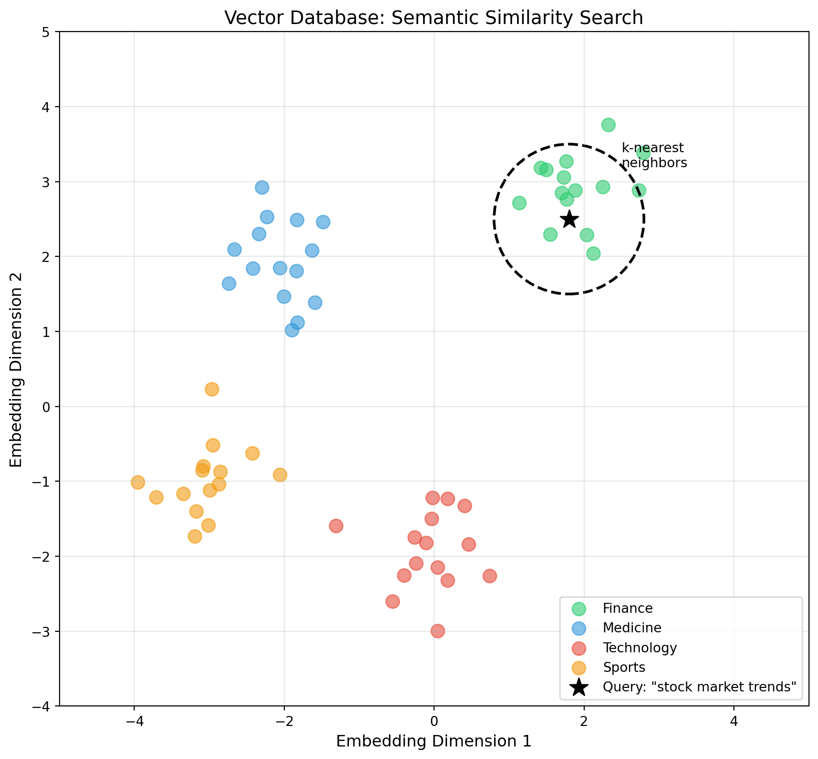
15.5.2 Vector Databases: The Foundation
A vector database is a specialized database optimized for storing, indexing, and querying high-dimensional vectors (embeddings). Unlike traditional databases that match exact values, vector databases find items that are semantically similar, meaning they’re close together in embedding space.
How Vector Databases Work
Embedding Generation: Convert documents, images, or other data into dense vectors using embedding models (like OpenAI’s
text-embedding-3, Cohere’s embeddings, or open-source models likebge-large)Indexing: Build data structures that enable fast approximate nearest neighbor (ANN) search. Exact search is O(n), which is impractical for millions of vectors. ANN algorithms trade small accuracy losses for dramatic speedups.
Querying: Convert the query to a vector, find the k most similar vectors in the index, and return the associated documents.
Approximate Nearest Neighbor (ANN) Algorithms
The core innovation enabling vector databases at scale:
HNSW (Hierarchical Navigable Small World): - Builds a multi-layer graph where each node connects to semantically similar neighbors - Search starts at the top layer (sparse, long-range connections) and descends to lower layers (dense, local connections) - Achieves O(log n) query time with high recall (>95%) - Used by Pinecone, Qdrant, Weaviate, pgvector
IVF (Inverted File Index): - Clusters vectors using k-means, then searches only relevant clusters - Faster indexing than HNSW, but lower recall for the same speed - Often combined with Product Quantization (IVF-PQ) for memory efficiency - Used by FAISS, Milvus
LSH (Locality-Sensitive Hashing): - Uses hash functions that map similar vectors to the same bucket - Fast but lower accuracy than HNSW/IVF - Better for very high-dimensional data
Major Vector Database Platforms
The vector database landscape has exploded, with options ranging from libraries to fully managed services:
FAISS (Facebook AI Similarity Search): - Open-source library (not a database) from Meta Research - Extremely fast, GPU-accelerated - No persistence, APIs, or management (you build those yourself) - Best for: Research, maximum performance, billions of vectors - Trade-off: Requires significant engineering
Pinecone: - Fully managed cloud service - Handles scaling, replication, and updates automatically - Simple API, metadata filtering, sparse-dense hybrid search - Best for: Production applications, minimal DevOps - Trade-off: Vendor lock-in, usage-based pricing
Weaviate: - Open-source with managed cloud option - Excels at hybrid search (combining vector + keyword + metadata) - GraphQL API, built-in vectorization modules - Best for: RAG applications needing flexible queries - Trade-off: More complex configuration
Qdrant: - Open-source, written in Rust for performance - Strong metadata filtering capabilities - Payload storage alongside vectors - Best for: When you need both similarity and complex filters - Trade-off: Smaller ecosystem than alternatives
Chroma: - Lightweight, developer-friendly - Designed for prototyping and small-scale applications - Best for: Getting started, local development - Trade-off: Not designed for large-scale production
pgvector: - PostgreSQL extension - Use existing PostgreSQL infrastructure - Best for: Teams already using PostgreSQL - Trade-off: Performance limitations at very large scale
TipNeuroscience Connection: Content-Addressable Memory in the Hippocampus
Vector databases implement a computational version of content-addressable memory, retrieving stored items based on similarity to a query pattern rather than an exact address. This is remarkably similar to how the hippocampus retrieves episodic memories.
The hippocampus uses pattern completion: a partial cue (a smell, a few words of a song) activates a stored memory trace, filling in the complete episode. This is analogous to a vector query: a semantically similar query retrieves documents that share meaning, even without matching keywords.
The brain’s memory retrieval also exhibits graceful degradation: similar cues retrieve similar memories. This is precisely what vector databases provide: queries that are “close” in embedding space return relevant results, even if the exact terms differ. The hippocampus achieves this through overlapping neural representations; vector databases achieve it through learned embeddings.
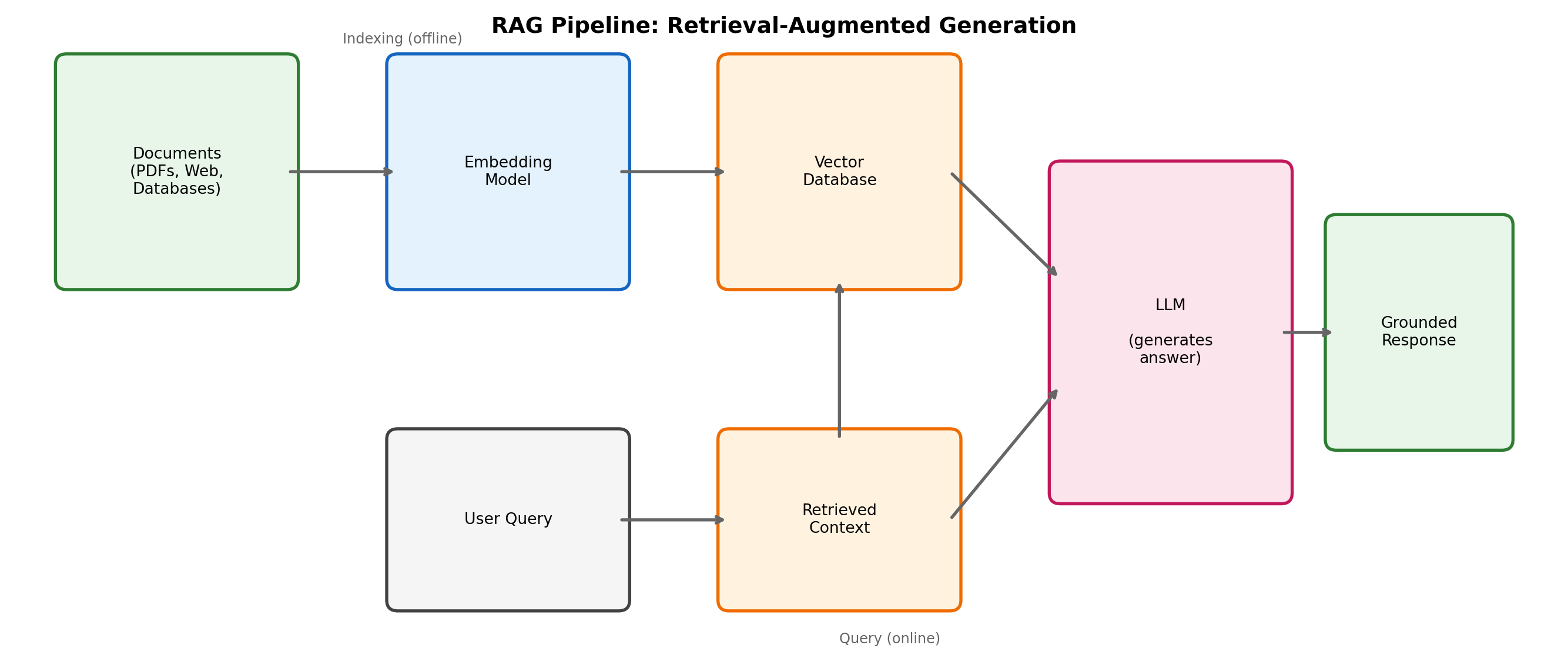
15.5.3 Retrieval-Augmented Generation (RAG)
RAG combines retrieval and generation: instead of relying solely on knowledge frozen in model weights, RAG systems retrieve relevant documents and include them in the LLM’s context, grounding responses in specific sources.
The RAG Pipeline
- Indexing Phase (offline):
- Split documents into chunks (paragraphs, sections, or semantic units)
- Generate embeddings for each chunk
- Store in vector database with metadata (source, date, etc.)
- Query Phase (online):
- Convert user query to embedding
- Retrieve top-k most similar chunks
- Construct prompt: system instructions + retrieved context + user question
- Generate response grounded in retrieved documents
Advanced RAG Techniques
Chunking Strategies: - Fixed-size: Simple but may split mid-sentence - Semantic: Use sentence boundaries or paragraph breaks - Recursive: Split large chunks until under size limit - Document-aware: Respect headers, sections, code blocks
Hybrid Search: - Combine dense vectors (semantic) with sparse vectors (keyword/BM25) - Captures both meaning similarity and exact term matches - Critical for technical domains with specific terminology
Reranking: - Initial retrieval returns many candidates quickly - A more powerful cross-encoder reranks the top results - Improves precision at the cost of latency
Query Transformation: - HyDE (Hypothetical Document Embedding): Generate a hypothetical answer, embed that instead of the question - Query expansion: Add synonyms and related terms - Multi-query: Generate multiple perspectives on the question
Agentic RAG: - The LLM decides when and what to retrieve - Can iterate: retrieve → reason → retrieve more if needed - Handles complex, multi-step questions
NoteRAG vs. Fine-tuning: When to Use Each
| Aspect | RAG | Fine-tuning |
|---|---|---|
| Knowledge updates | Instant (update documents) | Requires retraining |
| Source attribution | Can cite specific documents | Knowledge is implicit |
| Hallucination | Reduced (grounded in sources) | Still possible |
| Private data | Documents stay in your database | Data must be in training |
| Behavioral changes | Limited | Can change style, format |
| Cost | Per-query retrieval | One-time training cost |
Use RAG when: Knowledge changes frequently, sources must be cited, you have large document collections, or data privacy is critical.
Use fine-tuning when: You need to change the model’s behavior, style, or format; domain-specific vocabulary is essential; or consistent specialized knowledge is required.
Use both: Fine-tune for domain adaptation, then use RAG for specific, updatable knowledge.
15.5.4 Building Production RAG Systems
Moving from prototype to production requires addressing several challenges:
Evaluation: - Retrieval metrics: Precision@k, Recall@k, Mean Reciprocal Rank (MRR) - Generation metrics: Faithfulness (does the answer match retrieved context?), relevance, completeness - Human evaluation: Essential for subjective quality assessment
Scaling: - Index sharding across multiple nodes - Caching frequent queries - Async processing for batch operations
Monitoring: - Track retrieval latency and hit rates - Monitor embedding drift over time - Log failed retrievals for analysis
Security: - Access control at the document level - Prevent prompt injection through retrieved content - Audit trails for sensitive queries
The combination of vector databases and RAG has become the standard architecture for enterprise AI applications, enabling LLMs to access private, current, and verifiable knowledge while maintaining the flexibility and reasoning capabilities that make them powerful.
23.6 15.8 Limitations and Challenges
Despite their power, LLMs have significant limitations that are critical to understand for responsible application.
15.8.1 Hallucinations and Factuality
LLMs can generate text that is fluent, plausible, and completely false. This is called hallucination, and it’s perhaps the most critical risk for enterprise LLM deployment. Because models are trained to predict plausible sequences of text, not truthful ones, they can confidently invent facts, citations, events, or entire conversations that never happened.
Types of Hallucinations
Factual Hallucinations: - Inventing statistics: “Studies show that 73% of users prefer…” (no such study exists) - Creating false citations: “According to Smith et al. (2019) in Nature…” (paper doesn’t exist) - Wrong facts: “The Eiffel Tower was built in 1920” (it was 1889)
Entity Hallucinations: - Creating fictional people: “Dr. Sarah Mitchell at Stanford discovered…” - Mixing up real entities: Attributing one person’s work to another - Inventing organizations: “The International Board of AI Ethics states…”
Contextual Hallucinations: - Contradicting earlier statements in the same conversation - Making claims inconsistent with provided documents - Ignoring explicit user constraints
Structural Hallucinations: - Generating invalid code that looks syntactically plausible - Creating non-existent API endpoints or library functions - Producing malformed data structures
WarningThe Business Risk of Hallucinations
Hallucinations are not just academic concerns. They represent real business and legal risk:
- Legal liability: A lawyer was sanctioned for citing AI-generated fake case law
- Medical harm: Incorrect medical advice could injure patients
- Financial loss: Wrong financial data could lead to bad investment decisions
- Reputation damage: Publishing AI-generated falsehoods erodes trust
- Regulatory violations: Incorrect compliance information can lead to fines
For high-stakes applications, treating LLM outputs as “suggestions to be verified” rather than “facts to be trusted” is essential.
Why Do LLMs Hallucinate?
Training Objective Mismatch: LLMs are trained to predict likely text, not truthful text. If false information appears in training data, the model learns to reproduce it.
Compression of Knowledge: Billions of facts are compressed into model weights. Some get distorted or conflated, like a lossy JPEG with artifacts.
Pattern Completion Bias: When asked about obscure topics, the model fills in gaps with plausible-sounding patterns rather than admitting ignorance.
Confidence Calibration: Models aren’t trained to express uncertainty proportional to their actual knowledge.
Sycophancy: RLHF training can inadvertently reward models for agreeing with users, even when users are wrong.
Mitigation Strategies
1. Retrieval-Augmented Generation (RAG) (see Section 15.5): - Ground responses in retrieved, trusted documents - Model explicitly instructed to only use provided context - Can cite sources for verification - Limitation: Retrieval can fail; model may still hallucinate beyond context
2. Uncertainty Quantification: - Train models to output confidence scores - Use techniques like conformal prediction - Multiple model samples can indicate uncertainty (high variance = low confidence)
3. Fact-Checking Pipelines:
[LLM Response] → [Claim Extraction] → [Evidence Retrieval] → [Verification LLM] → [Flagged Output]- Extract factual claims from response
- Retrieve evidence for each claim
- Use separate model to verify claim against evidence
- Flag or filter unverified claims
4. Constrained Generation: - Restrict outputs to known-good formats (JSON schemas, SQL queries) - Use grammar-guided decoding - Post-generation validation
5. Prompt Engineering: - “If you don’t know, say ‘I don’t know’” - “Only provide information you’re certain about” - “Cite your sources for any claims” - Limitation: Models may ignore these instructions
6. Human-in-the-Loop: - For high-stakes decisions, require human verification - AI suggests, human approves - Escalation pathways for uncertain cases
TipNeuroscience Connection: Confabulation in the Brain
Hallucination has a biological analog: confabulation. Patients with certain brain injuries (especially to prefrontal cortex or basal forebrain) generate false memories with complete confidence, filling gaps in memory with plausible fabrications.
Key parallels: - Both involve generating plausible content without access to ground truth - Both show high confidence despite being factually wrong - Both reveal that “fluent generation” and “truthful generation” are separable
The brain normally relies on source monitoring (remembering where information came from) to distinguish real memories from imagined ones. LLMs lack this capability; they generate without tracking provenance. RAG partially addresses this by attaching sources to claims, implementing a form of artificial source monitoring.
15.8.2 Bias and Fairness
LLMs are trained on a snapshot of the internet, which is replete with human biases. Consequently, models can perpetuate and even amplify harmful stereotypes related to gender, race, religion, and other social categories.
Mitigation Strategies: - Data Curation: Carefully filtering and balancing the pre-training data to reduce exposure to biased content. - Alignment Tuning (RLHF): Using human feedback to train the model to avoid biased or stereotyped responses. - Red-Teaming: Adversarially probing the model to identify and patch vulnerabilities related to bias.
15.8.3 Context Window Limitations
The self-attention mechanism is computationally expensive, scaling quadratically with the length of the input sequence. This imposes a hard limit on the amount of text an LLM can consider at once, known as the context window. While recent models have expanded this to hundreds of thousands of tokens, it still falls short of processing an entire book or a large codebase in one go. This limits their ability to maintain coherence and recall information over very long interactions.
This section would contain hands-on code for fine-tuning and prompting.True23.7 15.6 Efficient Deployment: Quantization and Model Optimization
Training a 70-billion parameter model requires enormous resources, but running that model for inference doesn’t have to. Quantization and related techniques can shrink models by 4-8x while preserving most of their capabilities, enabling powerful AI on laptops, phones, and edge devices. This section covers the techniques that make small, efficient LLMs possible.
15.6.1 The GPS Analogy: Why Precision is Overrated
NoteThe In-N-Out Burger Test
Imagine you want to give a friend directions to In-N-Out Burger. You could provide GPS coordinates with 15 decimal places of precision:
Full precision (FP32): 34.019454238957123, -118.489234857234857
But that level of precision is absurd. It specifies a location down to the nanometer. Your friend doesn’t need to find a specific atom at In-N-Out; they need to find the building. Two decimal places is plenty:
Quantized (INT8-ish): 34.02, -118.49
With these “low precision” coordinates, your friend can see the restaurant and walk right in. The extra 13 decimal places were just wasted information. They made the coordinates harder to store and transmit without adding any practical value.
This is exactly what quantization does to neural network weights. Most of those 32 bits of precision in each weight are noise, not signal. We can throw away the unnecessary precision and keep only what matters for the model’s behavior.
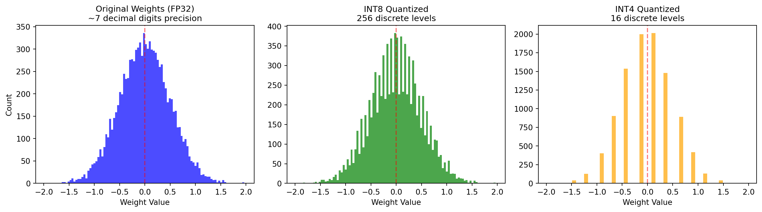
15.6.2 Understanding Numerical Precision
Neural networks traditionally store weights as 32-bit floating-point numbers (FP32). Each weight uses 32 bits of memory and can represent values with ~7 decimal digits of precision. But do we really need that precision?
The Number Formats:
| Format | Bits | Range | Precision | Memory per 7B model |
|---|---|---|---|---|
| FP32 | 32 | ±3.4×10³⁸ | ~7 digits | 28 GB |
| FP16 | 16 | ±65,504 | ~3 digits | 14 GB |
| BF16 | 16 | ±3.4×10³⁸ | ~3 digits | 14 GB |
| INT8 | 8 | -128 to 127 | 256 levels | 7 GB |
| INT4 | 4 | -8 to 7 | 16 levels | 3.5 GB |
Why Lower Precision Works:
Weight distributions are narrow: Most weights cluster around zero with small variance. We don’t need the full FP32 range.
Noise tolerance: Neural networks are trained with stochastic gradient descent, so they’re inherently robust to small perturbations. Rounding weights slightly doesn’t break them.
Redundancy: With billions of parameters, information is distributed across many weights. Small errors in individual weights average out.
The “dark matter” of weights: Studies show that many weights can be set to zero entirely (pruning) with minimal impact. If we can remove them completely, surely we can reduce their precision.
15.6.3 Quantization Techniques
Post-Training Quantization (PTQ): Apply quantization after training is complete. No retraining needed.
Absmax Quantization: Scale weights so the maximum absolute value maps to 127 (for INT8) \[w_{int8} = \text{round}\left(\frac{127 \cdot w}{max(|w|)}\right)\]
Zero-Point Quantization: Shift and scale to use the full range, handling asymmetric distributions
GPTQ: Advanced method that quantizes one layer at a time, using calibration data to minimize error
Quantization-Aware Training (QAT): Simulate quantization during training so the model learns to be robust to reduced precision. Produces better results but requires retraining.
Mixed-Precision Quantization: Not all layers are equally sensitive. Attention layers and the first/last layers often need higher precision. Modern quantization keeps critical layers in FP16 while aggressively quantizing feed-forward layers to INT4.
15.6.4 Practical Tools and Formats
The quantization ecosystem has standardized around several key tools and formats:
bitsandbytes: - Python library for 8-bit and 4-bit quantization - Integrates directly with Hugging Face Transformers - Enables loading models that wouldn’t otherwise fit in memory
# Load a 7B model in 4-bit precision (example syntax)
from transformers import AutoModelForCausalLM
model = AutoModelForCausalLM.from_pretrained(
    "meta-llama/Llama-2-7b-hf",
    load_in_4bit=True,
    device_map="auto"
)
# Model now uses ~3.5GB instead of ~28GB!
GGUF (GPT-Generated Unified Format): - File format designed for llama.cpp - Contains quantized weights + model metadata - Enables running models entirely on CPU - Common quantization levels: Q4_0, Q4_K_M, Q5_K_M, Q8_0
AWQ (Activation-aware Weight Quantization): - Identifies which weights are most important based on activation patterns - Protects important weights, aggressively quantizes less important ones - Often achieves better quality than uniform quantization
GGML/llama.cpp: - C/C++ library for CPU inference - Powers many local LLM applications - Runs quantized models efficiently without GPU
15.6.5 Quality vs. Size Trade-offs
How much quality do you lose? Less than you might think:
| Model | Format | Size | Perplexity | Relative Quality |
|---|---|---|---|---|
| Llama-2-7B | FP16 | 14 GB | 5.47 | 100% (baseline) |
| Llama-2-7B | Q8_0 | 7 GB | 5.48 | ~99.8% |
| Llama-2-7B | Q5_K_M | 4.8 GB | 5.52 | ~99% |
| Llama-2-7B | Q4_K_M | 4.1 GB | 5.58 | ~98% |
| Llama-2-7B | Q4_0 | 3.8 GB | 5.68 | ~96% |
The pattern is consistent: INT8 quantization is nearly lossless, and even INT4 preserves 95%+ of quality while reducing model size by 4x.
TipNeuroscience Connection: The Brain’s “Quantized” Representations
The brain doesn’t use infinite-precision representations either. Neural firing rates are inherently noisy, and information is encoded in population-level patterns rather than precise individual neuron activities.
Sparse Coding and Efficiency: The brain employs strategies remarkably similar to quantization: - Binary spikes: Neurons communicate with all-or-nothing action potentials (essentially a 1-bit signal) - Rate coding: Information is carried in firing rates, but with significant variability (noise) - Population codes: Meaning emerges from patterns across many neurons, averaging out individual noise
Studies of neural recordings show that relatively few bits per neuron are needed to decode behavior or stimuli. The brain achieves robust computation not through high-precision components, but through redundancy and error-tolerant coding. These are exactly the principles that make quantization work in neural networks.
Metabolic Efficiency: The brain consumes only ~20 watts while running a system far more capable than any AI. Part of this efficiency comes from “good enough” precision. Evolution optimized for metabolic efficiency, not numerical precision, and the result works remarkably well.
15.6.6 Model Merging: Combining Specialized Models
Beyond quantization, model merging offers another path to efficient, capable models: instead of training one large model, train (or fine-tune) specialized models and combine them.
Why Merge Models?
- Combine capabilities: Merge a model fine-tuned for coding with one fine-tuned for creative writing
- Average out biases: Merged models can be more balanced than individual fine-tunes
- No additional training: Merging happens post-hoc, requiring only arithmetic operations
Merging Techniques:
Linear Interpolation (LERP): Simply average the weights: \[W_{merged} = \alpha \cdot W_A + (1-\alpha) \cdot W_B\]
SLERP (Spherical Linear Interpolation): Interpolate along the surface of a hypersphere, preserving magnitude: \[W_{merged} = \frac{\sin((1-t)\theta)}{\sin\theta} W_A + \frac{\sin(t\theta)}{\sin\theta} W_B\]
SLERP often produces better results than linear interpolation because it respects the geometry of the weight space.
Task Arithmetic: Treat fine-tuning as adding a “task vector” to the base model: \[\tau = W_{fine-tuned} - W_{base}\] \[W_{new} = W_{base} + \alpha \cdot \tau_1 + \beta \cdot \tau_2\]
This allows combining multiple task-specific adaptations with controllable strengths.
TIES-Merging: Resolves conflicts when merging multiple models by: 1. Trimming small-magnitude changes (noise) 2. Resolving sign conflicts (when models disagree on direction) 3. Disjoint merging (averaging non-conflicting changes)
15.6.7 The Small Model Revolution
These efficiency techniques have enabled a revolution in accessible AI:
Running LLMs Locally: - A 7B model quantized to Q4 runs on a MacBook with 8GB RAM - A 3B model runs on smartphones - No internet connection, no API costs, complete privacy
The Efficiency Ladder:
| Use Case | Model Size | Quantization | Hardware | Latency |
|---|---|---|---|---|
| Cloud API | 70B+ | FP16 | 8×A100 | ~100ms |
| Workstation | 13-70B | Q4-Q8 | RTX 4090 | 50-200ms |
| Laptop | 7-13B | Q4-Q5 | M2 Mac | 100-500ms |
| Phone | 1-3B | Q4 | Snapdragon | 500ms-2s |
| Edge/IoT | <1B | Q4/INT8 | CPU | 1-5s |
Implications: - Privacy: Sensitive data never leaves the device - Latency: No network round-trip - Cost: No per-token API charges - Availability: Works offline, in remote areas - Customization: Fine-tune and merge for specific use cases
NoteThe Democratization of AI
Quantization and small models have democratized AI in ways that would have been unthinkable a few years ago. A student with a laptop can now run models comparable to what required a data center in 2020. The combination of efficient architectures, quantization techniques, and open-weight models has put powerful AI in everyone’s hands. This is a remarkable shift that’s changing who can build and benefit from these technologies.
23.8 15.7 Evaluating Language Model Performance
How do you know if an LLM is “good”? Unlike classification tasks with clear accuracy metrics, evaluating language models is surprisingly complex. Generated text can be fluent but factually wrong, or correct but awkwardly phrased. This section covers the metrics and methods used to evaluate LLM quality, which is essential knowledge for anyone fine-tuning or deploying these models.
15.7.1 The Evaluation Challenge
NoteWhy LLM Evaluation Is Hard
Consider this prompt: “Write a poem about autumn.”
A model might generate:
Leaves of amber, gold, and rust, Dancing on the morning gust, Summer’s warmth gives way to cold, Nature’s story, ages old.
Is this “good”? It depends on: - Fluency: Is the grammar correct? (Yes) - Coherence: Does it make sense? (Yes) - Creativity: Is it interesting? (Subjective) - Relevance: Is it about autumn? (Yes) - Originality: Is it plagiarized? (Need to check) - Style: Does it match the intended tone? (Depends)
No single number captures all these dimensions. This is why LLM evaluation combines multiple automated metrics with human judgment.
15.7.2 Perplexity: The Language Modeling Baseline
Perplexity is the most fundamental metric for language models. It measures how “surprised” the model is by a sequence of text. Lower is better.
Mathematical Definition:
\[\text{Perplexity}(X) = \exp\left(-\frac{1}{N}\sum_{i=1}^{N}\log P(x_i | x_1, ..., x_{i-1})\right)\]
where \(N\) is the number of tokens and \(P(x_i | ...)\) is the model’s predicted probability for token \(x_i\).
Interpretation: - Perplexity of 1: The model perfectly predicts every token (impossible in practice) - Perplexity of 10: On average, the model is as uncertain as if choosing from 10 equally likely options - Perplexity of 100: The model is quite uncertain
Typical Values: | Model | WikiText-2 Perplexity | |——-|———————-| | GPT-2 (124M) | 29.4 | | GPT-2 (1.5B) | 17.5 | | Llama-2 (7B) | 5.5 | | GPT-4 (est.) | <5 |
Limitations: - Only measures how well the model predicts held-out text - Doesn’t capture factuality, helpfulness, or style - A fluent but hallucinating model can have low perplexity
15.7.3 Text Similarity Metrics: BLEU and ROUGE
When you have reference text (e.g., a ground-truth translation or summary), you can measure how similar the generated text is to the reference.
BLEU (Bilingual Evaluation Understudy)
Originally designed for machine translation, BLEU measures n-gram overlap between generated and reference text.
How BLEU Works: 1. Count n-grams (1-grams, 2-grams, 3-grams, 4-grams) in both texts 2. Calculate precision: what fraction of generated n-grams appear in the reference? 3. Apply brevity penalty (prevents gaming by generating very short outputs) 4. Combine into a score from 0 to 1 (often reported as 0-100)
BLEU-4 Formula: \[\text{BLEU-4} = BP \cdot \exp\left(\sum_{n=1}^{4} w_n \log p_n\right)\]
where \(p_n\) is the n-gram precision, \(w_n = 0.25\) (equal weights), and \(BP\) is the brevity penalty.
Example: - Reference: “The cat sat on the mat.” - Generated: “The cat is sitting on the mat.” - Shared unigrams: “the” (2), “cat”, “on”, “mat” → High 1-gram precision - Shared bigrams: “the cat”, “on the” → Medium 2-gram precision - Result: BLEU ≈ 0.4-0.6 (reasonable but not perfect match)
Interpretation: | BLEU Score | Quality | |————|———| | < 10 | Almost useless | | 10-20 | Hard to understand | | 20-30 | Understandable, errors | | 30-40 | High quality | | 40-50 | Very high quality | | 50+ | Near professional |
ROUGE (Recall-Oriented Understudy for Gisting Evaluation)
While BLEU focuses on precision (is generated text in reference?), ROUGE emphasizes recall (is reference text in generation?). It’s preferred for summarization.
ROUGE Variants: - ROUGE-1: Unigram overlap (word-level) - ROUGE-2: Bigram overlap (captures some fluency) - ROUGE-L: Longest Common Subsequence (captures sequence structure) - ROUGE-Lsum: ROUGE-L over multiple sentences
ROUGE Formulas: \[\text{ROUGE-N Recall} = \frac{\text{Matching N-grams}}{\text{Total N-grams in Reference}}\]
\[\text{ROUGE-N Precision} = \frac{\text{Matching N-grams}}{\text{Total N-grams in Generation}}\]
\[\text{ROUGE-N F1} = 2 \times \frac{\text{Precision} \times \text{Recall}}{\text{Precision} + \text{Recall}}\]
When to Use Which: - BLEU: Translation, where you want generated text to be precise - ROUGE: Summarization, where you want to capture key information from the source
WarningThe Limitations of N-gram Metrics
BLEU and ROUGE were designed for an earlier era. They have significant blind spots:
Paraphrases: “The dog ran quickly” vs. “The canine sprinted fast” share no 2-grams despite identical meaning
Semantic similarity: “I love this movie” vs. “This film is wonderful” have low n-gram overlap but high semantic similarity
Factuality: A fluent but hallucinated response can score well if it uses similar words
Context insensitivity: Same n-grams in different contexts mean different things
Modern evaluation increasingly relies on learned metrics and human evaluation.
15.7.4 Semantic Similarity Metrics: BERTScore and Beyond
BERTScore addresses n-gram limitations by using contextual embeddings to compare meaning, not just surface forms.
How BERTScore Works: 1. Encode reference and generated text with BERT (or similar model) 2. For each token in generated text, find most similar token in reference (cosine similarity) 3. Aggregate into precision, recall, and F1 scores
Advantages: - Captures paraphrases and synonyms - Context-sensitive (same word, different meanings are handled) - Correlates better with human judgment than BLEU/ROUGE
Other Semantic Metrics: - MoverScore: Uses Word Mover’s Distance with contextualized embeddings - BLEURT: BERT fine-tuned on human ratings of text similarity - COMET: Trained on human translation quality judgments
15.7.5 Task-Specific Benchmarks
LLMs are evaluated on standardized benchmarks that test specific capabilities:
Reasoning and Knowledge: | Benchmark | Tests | Example Task | |———–|——-|————–| | MMLU | Multitask knowledge | 57 subjects from chemistry to law | | HellaSwag | Commonsense reasoning | Complete sentences plausibly | | ARC | Science questions | Grade school science | | TruthfulQA | Factuality | Avoid common misconceptions | | GSM8K | Math reasoning | Grade school word problems |
Coding: | Benchmark | Tests | Example Task | |———–|——-|————–| | HumanEval | Code generation | Write functions from docstrings | | MBPP | Python programming | Solve simple programming problems | | SWE-bench | Real-world coding | Fix actual GitHub issues |
Safety and Alignment: | Benchmark | Tests | Example Task | |———–|——-|————–| | MT-Bench | Multi-turn dialogue | Rate helpfulness over conversations | | AlpacaEval | Instruction following | Compare to reference model | | BBQ | Bias detection | Identify biased responses |
15.7.6 Human Evaluation: The Gold Standard
Automated metrics can only go so far. For nuanced quality assessment, human evaluation remains essential.
Common Approaches:
Likert Scale Ratings: - Fluency: Rate 1-5 how natural the text sounds - Coherence: Rate 1-5 how logical and organized it is - Helpfulness: Rate 1-5 how useful the response is - Harmlessness: Rate 1-5 how safe the response is
Pairwise Comparison (A/B Testing): - Show evaluators two responses - Ask: “Which is better?” (or “tie”) - More reliable than absolute ratings - Powers systems like Chatbot Arena’s Elo ratings
Elo Ratings for LLMs: The Chatbot Arena (LMSYS) runs a crowdsourced A/B test where users chat with anonymous models and vote on which is better. This produces Elo ratings similar to chess:
| Model | Elo (approx.) |
|---|---|
| GPT-4-turbo | 1250 |
| Claude 3 Opus | 1230 |
| Gemini Ultra | 1210 |
| Llama-3-70B | 1180 |
| GPT-3.5-turbo | 1100 |
Challenges with Human Evaluation: - Expensive and slow - Subjective (inter-annotator disagreement) - Doesn’t scale to continuous monitoring - Annotator fatigue affects quality
15.7.7 LLM-as-Judge: Using Models to Evaluate Models
A emerging paradigm uses strong LLMs to evaluate weaker ones:
# Example prompt for LLM-as-judge
evaluation_prompt = """
You are an expert evaluator. Rate the following response on a scale of 1-10.

Question: {question}
Response: {response}

Rate on:
1. Accuracy (is the information correct?)
2. Helpfulness (does it answer the question?)
3. Clarity (is it well-written?)

Provide scores and brief justification.
"""Advantages: - Fast and cheap at scale - Consistent (no annotator fatigue) - Can explain its reasoning
Limitations: - Biases of the judge model propagate - Self-preference (models rate their own outputs higher) - May miss subtle factual errors
Best Practice: Use LLM-as-judge for rapid iteration, validate important decisions with human evaluation.
TipNeuroscience Connection: How Do Humans Evaluate Language?
The brain’s evaluation of language quality involves multiple systems:
Fluency Processing (Broca’s Area): Grammatical violations trigger the P600 event-related potential, indicating syntactic processing. This is analogous to automated fluency checks.
Semantic Integration (Wernicke’s Area): Semantic anomalies trigger the N400 response. The brain constantly evaluates whether new words fit the semantic context, similar to how BERTScore measures contextual fit.
Pragmatic Evaluation (Prefrontal Cortex): Higher-level judgments (Is this helpful? Is this appropriate?) involve prefrontal regions that integrate context, goals, and social norms. This is what human evaluation captures but automated metrics miss.
Theory of Mind (TPJ, mPFC): Evaluating whether text will be understood by others requires modeling the reader’s knowledge state. Current metrics don’t explicitly do this, but humans naturally consider it.
The hierarchy of evaluation in the brain, from low-level fluency to high-level pragmatics, suggests that comprehensive LLM evaluation needs multiple metrics operating at different levels of abstraction.
15.7.8 Practical Evaluation Strategy
A comprehensive evaluation strategy combines multiple approaches:
For Fine-tuning Iteration: 1. Perplexity on validation set (quick feedback) 2. Task-specific metrics (BLEU, ROUGE, accuracy on benchmarks) 3. LLM-as-judge for qualitative assessment 4. Spot-check failures manually
For Pre-deployment: 1. Run standard benchmarks (MMLU, HumanEval, etc.) 2. Red-teaming for safety issues 3. A/B test against baseline with internal evaluators 4. Small-scale user study for real-world feedback
For Production Monitoring: 1. Track user engagement (thumbs up/down, regeneration requests) 2. Sample outputs for periodic human review 3. Monitor for regression on automated metrics 4. Collect and analyze failure cases
ImportantChapter Summary
In this chapter, we explored the revolutionary impact of Large Language Models on artificial intelligence:
- Transformer Architecture forms the foundation of modern LLMs, enabling unprecedented scale through efficient parallelization.
- Scaling Laws revealed that performance improves predictably with model size, dataset size, and compute, leading to the emergence of new capabilities at sufficient scale.
- Subword Tokenization (BPE, WordPiece) elegantly solves the vocabulary problem by learning to segment text into meaningful units that often correspond to morphemes, mirroring how the brain decomposes words during reading.
- Encoder Models (BERT) use bidirectional attention and masked language modeling to create deep contextual representations, excelling at understanding tasks where GPT-style decoders excel at generation.
- Pre-training Objectives like next-token prediction force models to develop rich world knowledge and reasoning abilities through self-supervised learning.
- Fine-tuning Methods including full fine-tuning, PEFT techniques like LoRA, and RLHF enable efficient adaptation of large models to specific tasks and alignment with human values.
- Prompting Techniques such as few-shot learning and chain-of-thought reasoning unlock latent capabilities without requiring weight updates.
- Vector Databases enable semantic similarity search over billions of embeddings, providing the infrastructure for retrieval-augmented generation (RAG) systems that ground LLM responses in external, updatable knowledge. This is analogous to the hippocampus’s content-addressable memory.
- Quantization and Model Optimization enable running powerful models on consumer hardware by reducing precision from 32-bit to 8-bit or 4-bit integers. The brain similarly achieves robust computation through “good enough” precision and redundancy rather than infinite accuracy.
- Model Merging techniques like SLERP and task arithmetic allow combining specialized fine-tunes without retraining, mirroring how the brain integrates multiple learned skills.
- Evaluation Metrics range from perplexity and n-gram overlap (BLEU, ROUGE) to semantic similarity (BERTScore) and human evaluation, reflecting the brain’s multi-level language assessment from syntax to pragmatics.
- Neural Parallels connect LLM mechanisms to brain language processing, including the predictive processing framework and hierarchical temporal representations.
- Limitations including hallucinations, bias, and context window constraints remain critical challenges for responsible deployment.
23.9 Exercises
Conceptual Questions
Emergent Abilities and Phase Transitions: The chapter describes how certain capabilities “emerge” suddenly when models cross a size threshold, rather than improving gradually. Explain this phenomenon using the concept of phase transitions from physics (e.g., water to steam). What does this suggest about the nature of intelligence and complexity? Are there analogous phenomena in brain development or evolution?
LoRA and Neural Modularity: LoRA enables efficient fine-tuning by training small adapter matrices while freezing the main model weights. How does this relate to the neuroscience concept of task-specific subnetworks? Discuss how the brain might implement similar modularity when learning new skills without catastrophic forgetting of old ones.
Chain-of-Thought and Dual Process Theory: The effectiveness of chain-of-thought prompting relates to Kahneman’s System 1 (fast, intuitive) vs. System 2 (slow, deliberate) thinking. Analyze this connection. What does the success of CoT prompting reveal about the computational requirements for complex reasoning? How might the brain implement similar sequential, explicit reasoning processes?
The Scaling Laws Paradox: Scaling laws suggest that simply making models bigger will continue to improve performance. However, the human brain has roughly the same number of neurons across adults. How can we reconcile the success of scaling in AI with the apparent lack of a “bigger brain = smarter human” relationship? What factors beyond raw parameter count might determine intelligence in biological systems?
Computational Problems
- Fine-Tuning a Small Language Model: Using a pre-trained model like GPT-2 (small) or BERT, implement instruction fine-tuning on a custom dataset:
- Create a dataset of instruction-response pairs for a specific domain (e.g., medical Q&A, code explanation, creative writing)
- Implement both full fine-tuning and LoRA-based fine-tuning
- Compare training time, memory usage, and performance
- Analyze examples where the model’s behavior changed after fine-tuning vs. examples where it retained general knowledge
- Test for catastrophic forgetting by evaluating on general benchmarks before and after fine-tuning
- Prompt Engineering Experiments: Design a systematic experiment to evaluate different prompting strategies:
- Choose a challenging reasoning task (e.g., multi-step math problems, logical puzzles, or scientific reasoning)
- Test zero-shot, few-shot (2, 4, 8 examples), and chain-of-thought prompting
- For CoT, compare manually written reasoning chains vs. asking the model to “think step by step”
- Quantify performance and analyze failure modes
- Identify which types of problems benefit most from each prompting strategy
- Analyzing Scaling Laws: Using a family of pre-trained models of different sizes (e.g., GPT-2 small, medium, large, XL):
- Evaluate perplexity on a held-out test set for each model size
- Plot loss vs. number of parameters on a log-log scale
- Fit a power law curve to your data
- Use your fitted curve to predict the performance of a hypothetical larger model
- Discuss limitations of extrapolating these curves beyond the observed range
- Building a Toy Reward Model for RLHF: Simulate the RLHF process on a small scale:
- Generate multiple responses to the same prompts using a small language model with different temperature settings
- Manually rank responses or create synthetic preference data
- Train a reward model to predict preference scores
- Analyze what features the reward model has learned (e.g., length, formality, factuality)
- Discuss how this reward model could be used to fine-tune the original LLM
Discussion Questions
Hallucinations and Epistemic Uncertainty: LLMs confidently generate false information. From a neuroscience perspective, discuss how humans calibrate confidence and express uncertainty. What mechanisms allow humans to know what they don’t know? Could similar metacognitive capabilities be built into LLMs? Propose specific architectural modifications or training objectives that might help LLMs better represent and communicate their uncertainty.
Bias, Fairness, and the Training Data Mirror: LLMs trained on internet text inherit societal biases. Discuss the philosophical and practical challenges this creates:
- Is it possible (or even desirable) to create a “neutral” language model?
- Should LLMs reflect society as it is, or as we think it should be?
- How do biases in LLMs compare to biases in human cognition (e.g., implicit associations, stereotypes)?
- What are the responsibilities of AI developers, and what technical interventions (data curation, RLHF, etc.) show the most promise for reducing harmful outputs?
- How should we balance safety measures against concerns about censorship and limiting model capabilities?
23.10 References
Bai, Y., Jones, A., Ndousse, K., Askell, A., Chen, A., DasSarma, N., Drain, D., Fort, S., Ganguli, D., Henighan, T., Joseph, N., Kadavath, S., Kernion, J., Conerly, T., El-Showk, S., Elhage, N., Hatfield-Dodds, Z., Hernandez, D., Hume, T., … Kaplan, J. (2022). Training a helpful and harmless assistant with reinforcement learning from human feedback. arXiv preprint arXiv:2204.05862. https://arxiv.org/abs/2204.05862
Brown, T. B., Mann, B., Ryder, N., Subbiah, M., Kaplan, J., Dhariwal, P., Neelakantan, A., Shyam, P., Sastry, G., Askell, A., Agarwal, S., Herbert-Voss, A., Krueger, G., Henighan, T., Child, R., Ramesh, A., Ziegler, D. M., Wu, J., Winter, C., … Amodei, D. (2020). Language models are few-shot learners. Advances in Neural Information Processing Systems, 33, 1877-1901. https://arxiv.org/abs/2005.14165
Christiano, P. F., Leike, J., Brown, T., Martic, M., Legg, S., & Amodei, D. (2017). Deep reinforcement learning from human preferences. Advances in Neural Information Processing Systems, 30. https://arxiv.org/abs/1706.03741
Devlin, J., Chang, M. W., Lee, K., & Toutanova, K. (2019). BERT: Pre-training of deep bidirectional transformers for language understanding. Conference of the North American Chapter of the Association for Computational Linguistics. https://arxiv.org/abs/1810.04805
Hu, E. J., Shen, Y., Wallis, P., Allen-Zhu, Z., Li, Y., Wang, S., Wang, L., & Chen, W. (2022). LoRA: Low-rank adaptation of large language models. International Conference on Learning Representations. https://arxiv.org/abs/2106.09685
Kaplan, J., McCandlish, S., Henighan, T., Brown, T. B., Chess, B., Child, R., Gray, S., Radford, A., Wu, J., & Amodei, D. (2020). Scaling laws for neural language models. arXiv preprint arXiv:2001.08361. https://arxiv.org/abs/2001.08361
Ouyang, L., Wu, J., Jiang, X., Almeida, D., Wainwright, C. L., Mishkin, P., Zhang, C., Agarwal, S., Slama, K., Ray, A., Schulman, J., Hilton, J., Kelton, F., Miller, L., Simens, M., Askell, A., Welinder, P., Christiano, P., Leike, J., & Lowe, R. (2022). Training language models to follow instructions with human feedback. Advances in Neural Information Processing Systems, 35. https://arxiv.org/abs/2203.02155
Radford, A., Narasimhan, K., Salimans, T., & Sutskever, I. (2018). Improving language understanding by generative pre-training. OpenAI. https://cdn.openai.com/research-covers/language-unsupervised/language_understanding_paper.pdf
Radford, A., Wu, J., Child, R., Luan, D., Amodei, D., & Sutskever, I. (2019). Language models are unsupervised multitask learners. OpenAI Blog, 1(8), 9. https://cdn.openai.com/better-language-models/language_models_are_unsupervised_multitask_learners.pdf
Schrimpf, M., Blank, I. A., Tuckute, G., Kauf, C., Hosseini, E. A., Kanwisher, N., Tenenbaum, J. B., & Fedorenko, E. (2021). The neural architecture of language: Integrative modeling converges on predictive processing. Proceedings of the National Academy of Sciences, 118(45), e2105646118. https://doi.org/10.1073/pnas.2105646118
Wei, J., Tay, Y., Bommasani, R., Raffel, C., Zoph, B., Borgeaud, S., Yogatama, D., Bosma, M., Zhou, D., Metzler, D., Chi, E. H., Hashimoto, T., Vinyals, O., Liang, P., Dean, J., & Fedus, W. (2022). Emergent abilities of large language models. Transactions on Machine Learning Research. https://arxiv.org/abs/2206.07682
Wei, J., Wang, X., Schuurmans, D., Bosma, M., Ichter, B., Xia, F., Chi, E., Le, Q., & Zhou, D. (2022). Chain-of-thought prompting elicits reasoning in large language models. Advances in Neural Information Processing Systems, 35. https://arxiv.org/abs/2201.11903