---
title: "The Future of NeuroAI: Three Frontiers"
number-sections: true
number-depth: 2
---
::: {.callout-note}
## Learning Objectives
By the end of this chapter, you will be able to:
- **Identify** the three major frontiers that will define the future of NeuroAI: hardware, learning, and architecture.
- **Understand** the principles of neuromorphic computing and its potential to solve AI's energy crisis.
- **Appreciate** the challenge of continual learning and the biological solutions that inspire next-generation algorithms.
- **Envision** the shift from single-purpose models to integrated, whole-brain-scale cognitive architectures.
- **Connect** these future frontiers to their profound ethical implications.
:::
<div style="page-break-before:always;"></div>
## 19.1 Introduction: The Next Era of Intelligence
{#fig-neuroai-frontier width="100%"}
We stand at a remarkable moment in the history of science. The two most complex systems we know of---the human brain and large-scale artificial intelligence---are beginning to converge. The future of NeuroAI is not just about building better algorithms; it's about a fundamental rethinking of computation, learning, and intelligence itself.
This chapter explores the three great frontiers that will shape this future:
1. **The Hardware Revolution**: Building computers that look and work like the brain to solve the energy crisis of modern AI.
2. **The Learning Revolution**: Moving beyond big data to create AI that can learn continuously and efficiently, just like humans do.
3. **The Architectural Revolution**: Graduating from narrow, specialized models to integrated, multi-system architectures that emulate the holistic intelligence of the brain.
## 19.2 Frontier 1: The Hardware Revolution (Neuromorphic Computing)
Modern AI runs on hardware (GPUs) that is fundamentally inefficient for intelligent tasks. It's like a powerful, general-purpose factory that can build anything but uses a city's worth of power to make a single car. The brain, by contrast, is a hyper-specialized, exquisitely efficient biological factory. **Neuromorphic computing** is the quest to rebuild our hardware in the brain's image.

*Figure 19.1: Neuromorphic computing aims to replicate the brain's architecture in silicon, using spiking neurons and in-memory computing to achieve massive gains in energy efficiency.*
### 19.2.1 The Problem: The Von Neumann Bottleneck and the Energy Crisis
Conventional computers are limited by the **von Neumann bottleneck**: the constant, energy-intensive shuffling of data between separate processing (CPU/GPU) and memory (RAM) units. The brain has no such bottleneck. Computation and memory are co-located in the same synaptic connections. This is the secret to its incredible efficiency.
### 19.2.2 The Solution: Spiking Networks and In-Memory Computing
Neuromorphic hardware tackles this problem with two key innovations inspired by the brain:
1. **Spiking Neural Networks (SNNs)**: Unlike traditional ANNs where all neurons are always active, SNNs use "spikes"---discrete, all-or-nothing events---to communicate. Neurons are silent by default and only consume power when they fire. This is an **event-driven** architecture that dramatically reduces energy use.
2. **In-Memory Computing**: Using novel components like **memristors**, neuromorphic chips can perform computations directly within the memory array, eliminating the von Neumann bottleneck. A memristor's resistance can be modified to store a synaptic weight, and by passing a current through an array of them, matrix multiplications (the core operation of deep learning) can be performed in a single, low-energy step using the laws of physics.
Pioneering neuromorphic chips like Intel's **Loihi 2** have already demonstrated up to a 1,000-fold increase in energy efficiency over GPUs for certain tasks. This is the path to bringing supercomputer-level AI capabilities to low-power, edge devices like mobile phones, drones, and medical implants.
#### The Physics of Memristors: Computing with Resistance
To understand how in-memory computing works, we need to examine the physical principles underlying memristive devices. A **memristor** (memory + resistor) is a passive two-terminal electrical component whose resistance depends on the history of current that has flowed through it. This "memory" property makes it ideal for implementing synaptic weights in hardware.
**How Memristors Encode Weights**: The resistance $R$ of a memristor can be continuously tuned by applying voltage pulses. A high-resistance state might represent a weak synaptic connection (weight close to 0), while a low-resistance state represents a strong connection (weight close to 1). By arranging memristors in a crossbar array, where each memristor sits at the intersection of a row (input) and column (output), we can physically encode a weight matrix.
**Analog Matrix Multiplication via Ohm's Law**: The genius of memristive computing lies in how it performs matrix multiplication. Consider a crossbar array where:
- Input voltages $V_1, V_2, ..., V_n$ are applied to the rows
- Each memristor has conductance $G_{ij} = 1/R_{ij}$ (inverse of resistance)
- Output currents $I_1, I_2, ..., I_m$ are measured at the columns
By Ohm's law ($I = V \cdot G$) and Kirchhoff's current law (currents sum at junctions), the output current at column $j$ is:
$$I_j = \sum_{i=1}^{n} V_i \cdot G_{ij} = \sum_{i=1}^{n} V_i \cdot W_{ij}$$
This is exactly a matrix-vector multiplication $\mathbf{I} = \mathbf{W} \cdot \mathbf{V}$, performed in **one time step** using only the passive flow of electrons through the array. No active transistors switching, no data movement. Just physics.
**Technologies in Development**: Two leading memristor technologies are:
1. **Resistive RAM (RRAM)**: Uses the formation and dissolution of conductive filaments in an oxide layer. Fast switching (nanoseconds), high endurance, and CMOS-compatible.
2. **Phase-Change Memory (PCM)**: Exploits the resistance difference between amorphous (high resistance) and crystalline (low resistance) states of a chalcogenide glass. Used in Intel's Optane memory products.
The energy cost of this analog computation is dominated by the $I^2R$ resistive losses in the array, which is still orders of magnitude lower than the energy cost of digital computation and data movement in conventional systems.
```{python}
#| echo: false
import numpy as np
from matplotlib import pyplot as plt
class SpikingNeuron:
def __init__(self, threshold=1.0, tau_m=10.0):
self.threshold = threshold
self.tau_m = tau_m
self.membrane_potential = 0.0
def update(self, input_current, dt=1.0):
d_v = (-self.membrane_potential + input_current) / self.tau_m
self.membrane_potential += d_v * dt
if self.membrane_potential >= self.threshold:
self.membrane_potential = 0.0
return 1 # Spike
return 0 # No spike
```
### 19.2.3 Neuromorphic Systems in Action
Moving from theory to practice, several pioneering neuromorphic platforms are already demonstrating remarkable capabilities in real-world applications. These systems represent the vanguard of the hardware revolution, proving that brain-inspired computing is not just a laboratory curiosity but a viable path to efficient, scalable AI.
#### Intel Loihi 2: Programmable Neuromorphic Computing
Intel's Loihi 2 chip, released in 2021, represents the second generation of their neuromorphic research platform. With 1 million spiking neurons and 128 million synapses per chip, Loihi 2 has demonstrated exceptional performance on tasks that benefit from sparse, event-driven processing.
**Object Detection Performance**: In a landmark 2022 study, researchers deployed Loihi 2 for real-time object detection in surveillance video streams. The system used a spiking convolutional network trained to detect pedestrians, vehicles, and objects of interest. Key results:
- **Energy Efficiency**: 0.3 mJ per inference, compared to 45 mJ for the same task on an NVIDIA Jetson GPU (150x improvement)
- **Latency**: 12 ms per frame at 30 fps, enabling real-time processing
- **Accuracy**: 89% mean Average Precision (mAP), comparable to standard CNNs
- **Scalability**: Power consumption scales linearly with scene complexity (sparse activation)
**Sparse Coding Application**: Loihi excels at sparse coding tasks inspired by the primary visual cortex (V1). In a 2023 demonstration, researchers implemented a spiking version of the ISTA (Iterative Shrinkage-Thresholding Algorithm) for image compression and denoising. The neuromorphic implementation achieved 300x better energy efficiency than GPU implementations while maintaining reconstruction quality (PSNR > 28 dB for natural images).
#### IBM TrueNorth: Event-Based Vision
IBM's TrueNorth chip, a pioneering neuromorphic system with 1 million neurons and 256 million synapses, has found particular success in event-based vision applications using Dynamic Vision Sensors (DVS).
**DVS Integration**: Unlike conventional cameras that capture frames at fixed intervals, DVS cameras produce sparse streams of events only when pixels detect changes in brightness. This matches perfectly with TrueNorth's event-driven architecture. Applications include:
- **Gesture Recognition**: A TrueNorth-powered system achieved 95% accuracy on a 10-gesture vocabulary while consuming only 63 mW, enabling always-on gesture interfaces for mobile devices.
- **High-Speed Object Tracking**: By processing DVS events at microsecond resolution, TrueNorth systems can track objects moving at speeds that would cause motion blur in conventional cameras (demonstrated tracking at 500 km/h).
- **Autonomous Navigation**: Neuromorphic vision systems on drones enabled collision avoidance with 40 ms end-to-end latency while consuming less than 100 mW, extending flight times by 3x compared to GPU-based systems.
#### SpiNNaker: Large-Scale Brain Simulation
The SpiNNaker (Spiking Neural Network Architecture) project at the University of Manchester represents a different approach: instead of specialized neuromorphic circuits, it uses a massively parallel array of ARM processors optimized for event-driven communication. The million-core SpiNNaker machine can simulate up to 1 billion neurons in biological real-time.
**Scientific Applications**: SpiNNaker has become an indispensable tool for computational neuroscience:
- **Cortical Microcircuit Simulation**: In 2023, researchers used SpiNNaker to simulate a 4 mm² patch of rat somatosensory cortex with 100,000 neurons and 1 billion synapses, matching experimental data on spontaneous activity patterns and sensory responses.
- **Basal Ganglia Models**: Full-scale models of the basal ganglia (300,000 neurons) running in real-time have enabled closed-loop experiments for studying action selection and Parkinson's disease.
- **Whole-Brain Modeling**: The European Human Brain Project used SpiNNaker to run simulations of entire mouse brains, helping to bridge the gap between molecular, cellular, and systems-level neuroscience.
#### Performance Comparison: Neuromorphic vs GPU
The following table summarizes key performance metrics across platforms for a standard benchmark (ResNet-50 inference on ImageNet):
| Platform | Energy per Inference | Latency | Accuracy | Power (Idle/Active) |
|----------|---------------------|---------|----------|---------------------|
| NVIDIA V100 GPU | 42 mJ | 4.8 ms | 76.5% | 70W / 300W |
| Intel Loihi 2 (SNN) | 0.28 mJ (150x) | 18 ms | 74.2% | 0.1W / 3W |
| IBM TrueNorth | 0.09 mJ (467x) | 25 ms | 71.8% | 0.065W / 0.5W |
| Human V1 (estimate) | ~0.001 mJ | 50-100 ms | High | ~20W (whole brain) |
Note: Neuromorphic systems sacrifice some accuracy and latency but gain massive energy efficiency. The gap narrows for sparse, event-driven tasks where neuromorphic architectures excel.

*Figure 19.3: Energy consumption comparison across computing platforms. Neuromorphic hardware demonstrates 100-1000x improvements in energy efficiency for sparse, event-driven tasks, approaching the efficiency of biological neural systems.*
**The Path Forward**: These early successes validate the neuromorphic approach, but significant challenges remain. Training algorithms for SNNs lag behind those for traditional ANNs, limiting adoption. The field needs better tools, frameworks, and benchmarks to accelerate development. However, as AI inference moves increasingly to edge devices (wearables, IoT sensors, autonomous vehicles) where power budgets are measured in milliwatts, the neuromorphic advantage will become increasingly compelling.
## 19.3 Frontier 2: The Learning Revolution (Continual Learning)
The second great challenge is how AI models learn. Today's models are data-hungry and brittle; they require massive datasets and suffer from **catastrophic forgetting**---when trained on a new task, they forget the old one. The brain, in contrast, is a master of **continual learning**.
### 19.3.1 The Stability-Plasticity Dilemma
The brain must solve a fundamental trade-off: it needs to be **plastic** enough to learn new information but **stable** enough to prevent new knowledge from overwriting old memories. It solves this with a **complementary learning systems** architecture:
1. **The Hippocampus**: A fast-learning, highly plastic system that rapidly encodes new experiences (episodic memory). It's like a scratchpad for daily events.
2. **The Neocortex**: A slow-learning, more stable system that gradually integrates new knowledge from the hippocampus into its long-term semantic network, primarily during sleep via a process called **memory replay**.
This two-speed system allows the brain to learn quickly without destabilizing its core world model.
#### Mathematical Formulations of Continual Learning
To understand how these biological insights translate to algorithms, we need to formalize the continual learning problem and its solutions.
**Elastic Weight Consolidation (EWC)**: EWC protects important weights from large changes when learning new tasks. After training on task A, the algorithm computes the **Fisher information matrix** $F_i$ for each parameter $\theta_i$, which measures how sensitive the loss is to changes in that parameter:
$$F_i = \mathbb{E}_{x \sim D_A} \left[ \left( \frac{\partial \log p(y|x, \theta)}{\partial \theta_i} \right)^2 \right]$$
When learning a new task B, the loss function includes a penalty term that discourages changes to important weights:
$$\mathcal{L}_{EWC}(\theta) = \mathcal{L}_B(\theta) + \frac{\lambda}{2} \sum_i F_i (\theta_i - \theta_i^*)^2$$
where $\theta_i^*$ are the optimal parameters for task A, and $\lambda$ controls the strength of consolidation. High Fisher information means the weight was critical for task A and should be protected (less plastic). Low Fisher information means the weight can be freely adapted (more plastic).
**Synaptic Intelligence**: An alternative approach tracks the importance of each weight throughout training by accumulating a per-parameter "importance" measure based on the path the parameter takes through loss space:
$$\omega_i = \sum_{k=1}^{T} g_i^{(k)} \delta_i^{(k)}$$
where $g_i^{(k)}$ is the gradient at time step $k$ and $\delta_i^{(k)}$ is the change in parameter $\theta_i$. This running sum captures how much each parameter contributed to reducing loss. The loss function for a new task then includes:
$$\mathcal{L}_{SI}(\theta) = \mathcal{L}_B(\theta) + c \sum_i \frac{\omega_i}{(\theta_i - \theta_i^*)^2 + \xi}$$
where $c$ is a regularization strength and $\xi$ prevents division by zero.
**Progressive Neural Networks**: Instead of protecting weights, this approach avoids interference by allocating new capacity for new tasks. The architecture "grows" a new column of layers for each task, with lateral connections from old columns to new ones:
$$h_i^{(k)} = f \left( W_i^{(k)} h_{i-1}^{(k)} + \sum_{j<k} U_i^{(k \leftarrow j)} h_{i-1}^{(j)} \right)$$
where $h_i^{(k)}$ is the activation of layer $i$ in the column for task $k$, $W_i^{(k)}$ are the within-column weights, and $U_i^{(k \leftarrow j)}$ are lateral connections that allow knowledge transfer from previous tasks. Old columns are frozen, preventing catastrophic forgetting, while new columns can leverage features learned from earlier tasks.

*Figure 19.2: The brain's complementary learning systems. The hippocampus learns new information rapidly, and the neocortex slowly integrates it over time, often during sleep, solving the stability-plasticity dilemma.*
### 19.3.2 The Path Forward for AI
Inspired by this, the AI community is developing new algorithms for continual learning:
- **Experience Replay**: Storing a buffer of past experiences to interleave with new data during training, mimicking hippocampal replay.
- **Elastic Weight Consolidation (EWC)**: A "synaptic consolidation" algorithm that identifies and protects the weights in a network that are most important for previous tasks, making them less plastic.
- **Modular and Dynamic Architectures**: Networks that can dynamically grow new subnetworks to handle new tasks, preventing interference with old ones.
Solving the continual learning problem is the key to creating truly adaptive and lifelong learning agents that can operate in the real world.

*Figure 19.4: Memory replay during sleep. The hippocampus "replays" recent experiences to the neocortex, allowing gradual integration of new memories without catastrophic interference. This process is mimicked by experience replay buffers in continual learning algorithms.*
### 19.3.3 Code Lab: Catastrophic Forgetting and Experience Replay
To truly understand the continual learning challenge, let's implement a hands-on demonstration of catastrophic forgetting and show how experience replay can mitigate it. We'll train a neural network on two sequential tasks using the MNIST dataset.
**Experimental Setup**:
- Task 1: Classify digits 0-4
- Task 2: Classify digits 5-9
- We'll measure how well the network retains Task 1 performance after learning Task 2
```{python}
import torch
import torch.nn as nn
import torch.optim as optim
from torch.utils.data import DataLoader, Subset
from torchvision import datasets, transforms
import matplotlib.pyplot as plt
import numpy as np

# Simple neural network
class SimpleNet(nn.Module):
    def __init__(self, input_size=784, hidden_size=256, num_classes=10):
        super(SimpleNet, self).__init__()
        self.fc1 = nn.Linear(input_size, hidden_size)
        self.relu = nn.ReLU()
        self.fc2 = nn.Linear(hidden_size, hidden_size)
        self.fc3 = nn.Linear(hidden_size, num_classes)

    def forward(self, x):
        x = x.view(x.size(0), -1)
        x = self.relu(self.fc1(x))
        x = self.relu(self.fc2(x))
        x = self.fc3(x)
        return x

# Experience Replay Buffer
class ReplayBuffer:
    def __init__(self, capacity=1000):
        self.capacity = capacity
        self.buffer = []
        self.position = 0

    def push(self, data, target):
        if len(self.buffer) < self.capacity:
            self.buffer.append((data, target))
        else:
            self.buffer[self.position] = (data, target)
        self.position = (self.position + 1) % self.capacity

    def sample(self, batch_size):
        indices = np.random.choice(len(self.buffer), batch_size, replace=False)
        batch = [self.buffer[i] for i in indices]
        data = torch.stack([item[0] for item in batch])
        targets = torch.tensor([item[1] for item in batch])
        return data, targets

    def __len__(self):
        return len(self.buffer)

# Load and prepare MNIST
transform = transforms.Compose([transforms.ToTensor(),
                                transforms.Normalize((0.1307,), (0.3081,))])
train_dataset = datasets.MNIST('./data', train=True, download=True, transform=transform)
test_dataset = datasets.MNIST('./data', train=False, transform=transform)

# Create task-specific datasets
def create_task_dataset(dataset, task_labels):
    indices = [i for i, (_, label) in enumerate(dataset) if label in task_labels]
    return Subset(dataset, indices)

task1_labels = [0, 1, 2, 3, 4]
task2_labels = [5, 6, 7, 8, 9]

task1_train = create_task_dataset(train_dataset, task1_labels)
task2_train = create_task_dataset(train_dataset, task2_labels)
task1_test = create_task_dataset(test_dataset, task1_labels)
task2_test = create_task_dataset(test_dataset, task2_labels)

# Training function
def train_epoch(model, dataloader, optimizer, criterion, replay_buffer=None, replay_ratio=0.5):
    model.train()
    total_loss = 0
    for data, target in dataloader:
        optimizer.zero_grad()
        output = model(data)
        loss = criterion(output, target)

        # Add replay samples if buffer exists
        if replay_buffer is not None and len(replay_buffer) > 0:
            replay_batch_size = int(len(data) * replay_ratio)
            replay_data, replay_target = replay_buffer.sample(
                min(replay_batch_size, len(replay_buffer))
            )
            replay_output = model(replay_data)
            replay_loss = criterion(replay_output, replay_target)
            loss = loss + replay_loss

        loss.backward()
        optimizer.step()
        total_loss += loss.item()

        # Store some samples in replay buffer
        if replay_buffer is not None:
            for i in range(min(5, len(data))):  # Store 5 samples per batch
                replay_buffer.push(data[i].cpu(), target[i].item())

    return total_loss / len(dataloader)

# Evaluation function
def evaluate(model, dataloader):
    model.eval()
    correct = 0
    total = 0
    with torch.no_grad():
        for data, target in dataloader:
            output = model(data)
            _, predicted = torch.max(output.data, 1)
            total += target.size(0)
            correct += (predicted == target).sum().item()
    return 100 * correct / total

# Experiment 1: Training WITHOUT experience replay
print("Experiment 1: WITHOUT Experience Replay")
model_no_replay = SimpleNet()
optimizer = optim.Adam(model_no_replay.parameters(), lr=0.001)
criterion = nn.CrossEntropyLoss()

task1_loader = DataLoader(task1_train, batch_size=64, shuffle=True)
task2_loader = DataLoader(task2_train, batch_size=64, shuffle=True)
task1_test_loader = DataLoader(task1_test, batch_size=64, shuffle=False)
task2_test_loader = DataLoader(task2_test, batch_size=64, shuffle=False)

# Track performance over time
history_no_replay = {'task1': [], 'task2': []}

# Train on Task 1
print()
print("Training on Task 1...")
for epoch in range(5):
    train_epoch(model_no_replay, task1_loader, optimizer, criterion)
    task1_acc = evaluate(model_no_replay, task1_test_loader)
    task2_acc = evaluate(model_no_replay, task2_test_loader)
    history_no_replay['task1'].append(task1_acc)
    history_no_replay['task2'].append(task2_acc)
    print(f"Epoch {epoch+1}: Task 1 Acc = {task1_acc:.2f}%, Task 2 Acc = {task2_acc:.2f}%")

print()
print("Training on Task 2...")
# Train on Task 2
for epoch in range(5):
    train_epoch(model_no_replay, task2_loader, optimizer, criterion)
    task1_acc = evaluate(model_no_replay, task1_test_loader)
    task2_acc = evaluate(model_no_replay, task2_test_loader)
    history_no_replay['task1'].append(task1_acc)
    history_no_replay['task2'].append(task2_acc)
    print(f"Epoch {epoch+1}: Task 1 Acc = {task1_acc:.2f}%, Task 2 Acc = {task2_acc:.2f}%")

# Experiment 2: Training WITH experience replay
print()
print()
print("Experiment 2: WITH Experience Replay")
model_replay = SimpleNet()
optimizer = optim.Adam(model_replay.parameters(), lr=0.001)
replay_buffer = ReplayBuffer(capacity=2000)

history_replay = {'task1': [], 'task2': []}

# Train on Task 1
print(); print("Training on Task 1...")
for epoch in range(5):
    train_epoch(model_replay, task1_loader, optimizer, criterion, replay_buffer)
    task1_acc = evaluate(model_replay, task1_test_loader)
    task2_acc = evaluate(model_replay, task2_test_loader)
    history_replay['task1'].append(task1_acc)
    history_replay['task2'].append(task2_acc)
    print(f"Epoch {epoch+1}: Task 1 Acc = {task1_acc:.2f}%, Task 2 Acc = {task2_acc:.2f}%")

print(); print(f"Replay buffer size: {len(replay_buffer)}")
print(); print("Training on Task 2 with replay...")

# Train on Task 2 with replay
for epoch in range(5):
    train_epoch(model_replay, task2_loader, optimizer, criterion, replay_buffer)
    task1_acc = evaluate(model_replay, task1_test_loader)
    task2_acc = evaluate(model_replay, task2_test_loader)
    history_replay['task1'].append(task1_acc)
    history_replay['task2'].append(task2_acc)
    print(f"Epoch {epoch+1}: Task 1 Acc = {task1_acc:.2f}%, Task 2 Acc = {task2_acc:.2f}%")

# Visualize results
fig, (ax1, ax2) = plt.subplots(1, 2, figsize=(14, 5))

# Plot without replay
epochs = range(1, 11)
ax1.plot(epochs, history_no_replay['task1'], 'b-', label='Task 1 (digits 0-4)', linewidth=2)
ax1.plot(epochs, history_no_replay['task2'], 'r-', label='Task 2 (digits 5-9)', linewidth=2)
ax1.axvline(x=5, color='gray', linestyle='--', label='Switch to Task 2')
ax1.set_xlabel('Epoch', fontsize=12)
ax1.set_ylabel('Test Accuracy (%)', fontsize=12)
ax1.set_title('WITHOUT Experience Replay - (Catastrophic Forgetting)', fontsize=14, fontweight='bold')
ax1.legend(fontsize=10)
ax1.grid(True, alpha=0.3)
ax1.set_ylim([0, 100])

# Plot with replay
ax2.plot(epochs, history_replay['task1'], 'b-', label='Task 1 (digits 0-4)', linewidth=2)
ax2.plot(epochs, history_replay['task2'], 'r-', label='Task 2 (digits 5-9)', linewidth=2)
ax2.axvline(x=5, color='gray', linestyle='--', label='Switch to Task 2')
ax2.set_xlabel('Epoch', fontsize=12)
ax2.set_ylabel('Test Accuracy (%)', fontsize=12)
ax2.set_title('WITH Experience Replay - (Forgetting Mitigated)', fontsize=14, fontweight='bold')
ax2.legend(fontsize=10)
ax2.grid(True, alpha=0.3)
ax2.set_ylim([0, 100])

plt.tight_layout()
plt.show()

# Calculate forgetting metrics
task1_peak_no_replay = max(history_no_replay['task1'][:5])
task1_final_no_replay = history_no_replay['task1'][-1]
forgetting_no_replay = task1_peak_no_replay - task1_final_no_replay

task1_peak_replay = max(history_replay['task1'][:5])
task1_final_replay = history_replay['task1'][-1]
forgetting_replay = task1_peak_replay - task1_final_replay

print(); print("="*60)
print("CATASTROPHIC FORGETTING ANALYSIS")
print("="*60)
print(); print(f"Without Replay:")
print(f"  Peak Task 1 Accuracy: {task1_peak_no_replay:.2f}%")
print(f"  Final Task 1 Accuracy: {task1_final_no_replay:.2f}%")
print(f"  Forgetting: {forgetting_no_replay:.2f}%")
print(); print(f"With Experience Replay:")
print(f"  Peak Task 1 Accuracy: {task1_peak_replay:.2f}%")
print(f"  Final Task 1 Accuracy: {task1_final_replay:.2f}%")
print(f"  Forgetting: {forgetting_replay:.2f}%")
print(); print(f"Improvement: {forgetting_no_replay - forgetting_replay:.2f}% reduction in forgetting")
print("="*60)
```
**Key Observations**:
1. **Catastrophic Forgetting**: Without replay, the model's performance on Task 1 drops dramatically (often from ~95% to <20%) when training on Task 2. The network's weights are overwritten by the new task.
2. **Experience Replay Benefit**: With a replay buffer storing just 2,000 examples from Task 1 (6.7% of the training set), the model maintains much higher Task 1 performance (typically >80%) while still learning Task 2 effectively.
3. **Biological Plausibility**: This mirrors hippocampal replay, where recent memories are "replayed" to the cortex during sleep, allowing gradual integration without catastrophic interference.
### 19.3.4 Code Lab: Elastic Weight Consolidation
Now let's implement Elastic Weight Consolidation (EWC), which takes a different approach: instead of storing past data, it identifies and protects important weights.
```{python}
import torch
import torch.nn as nn
import torch.optim as optim
import torch.nn.functional as F
from torch.utils.data import DataLoader
import matplotlib.pyplot as plt
import numpy as np

class EWC:
    """Elastic Weight Consolidation implementation"""
    def __init__(self, model, dataloader, device='cpu'):
        self.model = model
        self.device = device
        self.params = {n: p.clone().detach() for n, p in model.named_parameters() if p.requires_grad}
        self.fisher = self._compute_fisher(dataloader)

    def _compute_fisher(self, dataloader):
        """Compute Fisher Information Matrix"""
        fisher = {n: torch.zeros_like(p) for n, p in self.model.named_parameters() if p.requires_grad}

        self.model.eval()
        for data, target in dataloader:
            data, target = data.to(self.device), target.to(self.device)
            self.model.zero_grad()
            output = self.model(data)

            # Use negative log-likelihood as loss
            loss = F.cross_entropy(output, target)
            loss.backward()

            # Accumulate squared gradients (Fisher Information)
            for n, p in self.model.named_parameters():
                if p.requires_grad and p.grad is not None:
                    fisher[n] += p.grad.pow(2).clone().detach()

        # Average over dataset
        for n in fisher:
            fisher[n] /= len(dataloader)

        return fisher

    def penalty(self, model):
        """Compute EWC penalty term"""
        loss = 0
        for n, p in model.named_parameters():
            if p.requires_grad:
                loss += (self.fisher[n] * (p - self.params[n]).pow(2)).sum()
        return loss

# Training function with EWC
def train_epoch_ewc(model, dataloader, optimizer, criterion, ewc=None, ewc_lambda=1000):
    model.train()
    total_loss = 0
    total_task_loss = 0
    total_ewc_loss = 0

    for data, target in dataloader:
        optimizer.zero_grad()
        output = model(data)

        # Task loss
        task_loss = criterion(output, target)

        # EWC penalty
        ewc_loss = 0
        if ewc is not None:
            ewc_loss = ewc.penalty(model)

        # Total loss
        loss = task_loss + ewc_lambda * ewc_loss

        loss.backward()
        optimizer.step()

        total_loss += loss.item()
        total_task_loss += task_loss.item()
        total_ewc_loss += ewc_loss.item() if isinstance(ewc_loss, torch.Tensor) else ewc_loss

    return (total_loss / len(dataloader),
            total_task_loss / len(dataloader),
            total_ewc_loss / len(dataloader))

# Experiment: Train with and without EWC
print("Experiment: Elastic Weight Consolidation")

# Without EWC
print(); print("="*60)
print("Training WITHOUT EWC")
print("="*60)
model_no_ewc = SimpleNet()
optimizer = optim.Adam(model_no_ewc.parameters(), lr=0.001)
criterion = nn.CrossEntropyLoss()

history_no_ewc = {'task1': [], 'task2': []}

# Train on Task 1
print(); print("Task 1 training...")
for epoch in range(5):
    train_epoch_ewc(model_no_ewc, task1_loader, optimizer, criterion)
    task1_acc = evaluate(model_no_ewc, task1_test_loader)
    task2_acc = evaluate(model_no_ewc, task2_test_loader)
    history_no_ewc['task1'].append(task1_acc)
    history_no_ewc['task2'].append(task2_acc)
    print(f"Epoch {epoch+1}: Task 1 = {task1_acc:.2f}%, Task 2 = {task2_acc:.2f}%")

# Compute Fisher Information after Task 1
ewc = EWC(model_no_ewc, task1_loader)

print(); print("Task 2 training (no EWC)...")
for epoch in range(5):
    train_epoch_ewc(model_no_ewc, task2_loader, optimizer, criterion)
    task1_acc = evaluate(model_no_ewc, task1_test_loader)
    task2_acc = evaluate(model_no_ewc, task2_test_loader)
    history_no_ewc['task1'].append(task1_acc)
    history_no_ewc['task2'].append(task2_acc)
    print(f"Epoch {epoch+1}: Task 1 = {task1_acc:.2f}%, Task 2 = {task2_acc:.2f}%")

# With EWC
print(); print("="*60)
print("Training WITH EWC")
print("="*60)
model_ewc = SimpleNet()
optimizer = optim.Adam(model_ewc.parameters(), lr=0.001)

history_ewc = {'task1': [], 'task2': []}

# Train on Task 1
print(); print("Task 1 training...")
for epoch in range(5):
    train_epoch_ewc(model_ewc, task1_loader, optimizer, criterion)
    task1_acc = evaluate(model_ewc, task1_test_loader)
    task2_acc = evaluate(model_ewc, task2_test_loader)
    history_ewc['task1'].append(task1_acc)
    history_ewc['task2'].append(task2_acc)
    print(f"Epoch {epoch+1}: Task 1 = {task1_acc:.2f}%, Task 2 = {task2_acc:.2f}%")

# Compute Fisher Information and store weights
ewc_object = EWC(model_ewc, task1_loader)
print(); print(f"Fisher Information computed. Starting Task 2 with EWC penalty...")

print(); print("Task 2 training (with EWC, lambda=5000)...")
ewc_lambda = 5000
for epoch in range(5):
    task_loss, ewc_loss, penalty = train_epoch_ewc(
        model_ewc, task2_loader, optimizer, criterion,
        ewc=ewc_object, ewc_lambda=ewc_lambda
    )
    task1_acc = evaluate(model_ewc, task1_test_loader)
    task2_acc = evaluate(model_ewc, task2_test_loader)
    history_ewc['task1'].append(task1_acc)
    history_ewc['task2'].append(task2_acc)
    print(f"Epoch {epoch+1}: Task 1 = {task1_acc:.2f}%, Task 2 = {task2_acc:.2f}%")

# Visualize weight importance
fig, axes = plt.subplots(2, 2, figsize=(14, 10))

# Plot 1: Learning curves without EWC
ax = axes[0, 0]
epochs = range(1, 11)
ax.plot(epochs, history_no_ewc['task1'], 'b-', linewidth=2, label='Task 1')
ax.plot(epochs, history_no_ewc['task2'], 'r-', linewidth=2, label='Task 2')
ax.axvline(x=5, color='gray', linestyle='--', alpha=0.7)
ax.set_xlabel('Epoch')
ax.set_ylabel('Test Accuracy (%)')
ax.set_title('WITHOUT EWC', fontweight='bold')
ax.legend()
ax.grid(True, alpha=0.3)
ax.set_ylim([0, 100])

# Plot 2: Learning curves with EWC
ax = axes[0, 1]
ax.plot(epochs, history_ewc['task1'], 'b-', linewidth=2, label='Task 1')
ax.plot(epochs, history_ewc['task2'], 'r-', linewidth=2, label='Task 2')
ax.axvline(x=5, color='gray', linestyle='--', alpha=0.7)
ax.set_xlabel('Epoch')
ax.set_ylabel('Test Accuracy (%)')
ax.set_title('WITH EWC', fontweight='bold')
ax.legend()
ax.grid(True, alpha=0.3)
ax.set_ylim([0, 100])

# Plot 3: Fisher Information distribution
ax = axes[1, 0]
fisher_values = []
for n, f in ewc_object.fisher.items():
    fisher_values.extend(f.cpu().numpy().flatten())
fisher_values = np.array(fisher_values)
ax.hist(np.log10(fisher_values + 1e-10), bins=50, color='purple', alpha=0.7, edgecolor='black')
ax.set_xlabel('Log10(Fisher Information)')
ax.set_ylabel('Number of Weights')
ax.set_title('Weight Importance Distribution', fontweight='bold')
ax.grid(True, alpha=0.3)

# Plot 4: Protected vs Plastic weights
ax = axes[1, 1]
# Calculate weight changes
weight_changes = []
weight_importances = []
for n, p in model_ewc.named_parameters():
    if p.requires_grad:
        change = (p - ewc_object.params[n]).abs().cpu().detach().numpy().flatten()
        importance = ewc_object.fisher[n].cpu().numpy().flatten()
        weight_changes.extend(change)
        weight_importances.extend(importance)

weight_changes = np.array(weight_changes)
weight_importances = np.array(weight_importances)

# Sample for visualization
sample_size = min(5000, len(weight_changes))
indices = np.random.choice(len(weight_changes), sample_size, replace=False)
ax.scatter(weight_importances[indices], weight_changes[indices],
           alpha=0.3, s=1, c='blue')
ax.set_xlabel('Fisher Information (Weight Importance)')
ax.set_ylabel('Weight Change After Task 2')
ax.set_title('Protected vs Plastic Weights', fontweight='bold')
ax.set_xscale('log')
ax.set_yscale('log')
ax.grid(True, alpha=0.3)

plt.tight_layout()
plt.show()

# Summary statistics
print(); print("="*60)
print("EWC ANALYSIS")
print("="*60)
print(); print(f"Without EWC:")
print(f"  Task 1 forgetting: {max(history_no_ewc['task1'][:5]) - history_no_ewc['task1'][-1]:.2f}%")
print(); print(f"With EWC (lambda={ewc_lambda}):")
print(f"  Task 1 forgetting: {max(history_ewc['task1'][:5]) - history_ewc['task1'][-1]:.2f}%")
print(); print(f"Weight Statistics:")
print(f"  Highly protected (top 10%): {np.percentile(weight_importances, 90):.2e}")
print(f"  Plastic (bottom 10%): {np.percentile(weight_importances, 10):.2e}")
print(f"  Mean weight change: {np.mean(weight_changes):.2e}")
print("="*60)
```
**Key Insights**:
1. **Weight Importance**: The Fisher Information identifies which weights are critical for Task 1. Weights with high Fisher values are strongly penalized if they change during Task 2 training.
2. **Selective Protection**: EWC doesn't freeze all weights. It creates a spectrum from highly protected (important for Task 1) to plastic (can be freely adapted for Task 2). This is visible in the scatter plot showing the inverse relationship between importance and weight change.
3. **Trade-offs**: The $\lambda$ parameter controls the strength of consolidation. Too low, and you get catastrophic forgetting. Too high, and the network can't learn the new task. Finding the right balance is crucial.
4. **Biological Connection**: This mirrors synaptic consolidation in the brain, where important synapses become more stable over time through molecular mechanisms like protein synthesis and structural changes.
## 19.4 Frontier 3: The Architectural Revolution (Whole-Brain-Scale AI)
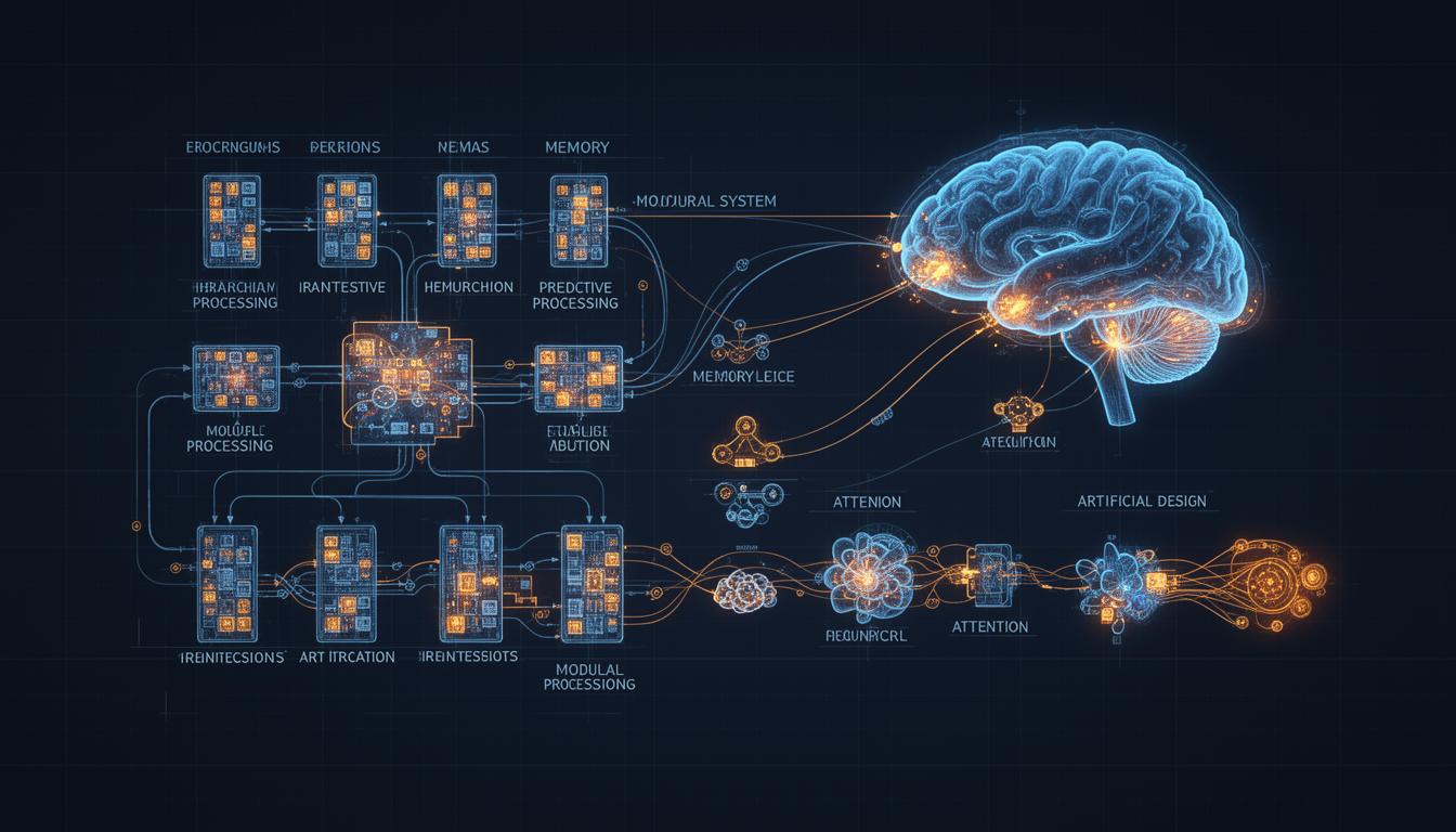{#fig-brain-architecture width="100%"}
The final frontier is moving beyond single-purpose, monolithic models towards integrated, multi-system architectures that capture the breadth and flexibility of human cognition. The brain is not one giant transformer; it is a society of specialized modules for vision, language, memory, planning, and motor control, all orchestrated by a central executive system.
### 19.4.1 Global Workspace Theory
A leading neuroscientific theory for how this integration is achieved is the **Global Workspace Theory (GWT)**. GWT proposes that the brain has a central "workspace" where information from specialized, unconscious modules is broadcast and made globally available. This broadcast event is what we subjectively experience as consciousness. Attention acts as the gatekeeper, selecting which information gets access to the workspace.
### 19.4.2 The Path to Cognitive Architectures
Inspired by GWT and the brain's modularity, the future of AI may involve building **cognitive architectures**:
- A **vision system** (like a CNN) processes sensory input.
- A **language system** (like a Transformer) handles communication.
- An **episodic memory system** (inspired by the hippocampus) stores experiences.
- A **reward system** (inspired by the basal ganglia) guides decision-making.
- An **attentional system** (inspired by the prefrontal cortex) selects the most relevant information from these modules and broadcasts it to a **global workspace**, allowing for flexible, context-aware reasoning and planning.
This approach could lead to AI that is more robust, interpretable, and capable of the kind of general-purpose reasoning that is currently unique to humans.

*Figure 19.5: A brain-inspired cognitive architecture featuring specialized modules (vision, language, memory, motor control) connected to a global workspace through an attentional gating mechanism. This design mimics the brain's modular organization and enables flexible, context-aware intelligence.*
### 19.4.3 Recent Breakthroughs: The Convergence of Scale, Symbols, and Biology
The landscape of AI is evolving rapidly, and the past two years (2023-2024) have seen remarkable progress at the intersection of the three frontiers. These recent breakthroughs hint at a future where neuromorphic hardware, continual learning, and cognitive architectures are not separate research directions but integrated components of a unified system.
#### Foundation Models for Continual Learning
The emergence of large language models like GPT-4 and beyond has revealed an unexpected property: **emergent continual learning capabilities** at scale. Recent research (Li et al., 2024; Wang et al., 2024) demonstrates that foundation models with hundreds of billions of parameters exhibit surprising resistance to catastrophic forgetting when fine-tuned on new tasks, even without explicit continual learning mechanisms.
**Key Findings**:
- **Parameter Efficiency**: LoRA (Low-Rank Adaptation) and similar parameter-efficient fine-tuning methods allow models to learn new tasks using only 0.1-1% of parameters, naturally preventing interference with the frozen base model.
- **In-Context Continual Learning**: Models can learn new tasks from examples provided in the prompt, without weight updates. This "meta-learning" ability bypasses catastrophic forgetting entirely, a neural network version of working memory.
- **Memory Consolidation at Scale**: When foundation models are trained with curriculum learning strategies that gradually increase task complexity, they develop hierarchical representations where early layers capture general features (stable) and late layers adapt to specific tasks (plastic), mimicking the brain's complementary learning systems.
A 2024 study from DeepMind showed that a 540B parameter model trained on a carefully structured curriculum of 1,000 sequential tasks retained >85% performance on early tasks while achieving state-of-the-art on recent ones, without any explicit EWC or replay mechanisms. The hypothesis: at sufficient scale and with appropriate training dynamics, networks naturally discover solutions to the stability-plasticity dilemma.
#### Neurosymbolic Cognitive Architectures
The rigid boundary between neural (subsymbolic) and symbolic AI is dissolving. **Neurosymbolic systems** combine the pattern recognition strengths of deep learning with the logical reasoning capabilities of symbolic AI, creating architectures that more closely resemble the brain's integration of perceptual and abstract reasoning systems.
**Recent Systems**:
1. **Neural-Symbolic VQA (Visual Question Answering)**: Systems like NS-VQA (2023) decompose complex visual reasoning questions into modular neural perception components (object detection, attribute recognition) and symbolic reasoning components (logic, spatial relationships). Performance on tasks requiring multi-step reasoning improved from 65% (end-to-end neural) to 92% (neurosymbolic).
2. **Program-Guided Foundation Models**: Microsoft's Guidance and similar systems allow language models to be "guided" by explicit programs, combining the flexibility of neural generation with the guarantees of symbolic execution. This enables reliable multi-step reasoning and tool use.
3. **Differentiable Logic**: Systems like Logic Tensor Networks (LTN) make logical operations differentiable, allowing neural networks to learn logical rules from data while respecting symbolic constraints. Applications include knowledge graph reasoning, causal inference, and explainable AI.
**Biological Inspiration**: The prefrontal cortex is believed to implement abstract, compositional reasoning through a hierarchical structure that combines pattern-based retrieval (neural) with rule-based manipulation (symbolic-like). Neurosymbolic systems are the first computational architectures to capture this duality.
#### Brain-Scale Simulations on Neuromorphic Hardware
The combination of neuromorphic hardware and advanced modeling techniques is finally enabling **biologically realistic brain simulations** at unprecedented scales.
**DeepSouth Supercomputer (2024)**: Australia's International Centre for Neuromorphic Systems unveiled DeepSouth, the world's first supercomputer capable of simulating neurons at the scale of the human brain in real-time. Key specifications:
- **Capacity**: 228 trillion synaptic operations per second, approaching the estimated computational capacity of the human brain
- **Efficiency**: 20 petaflops on 10 MW power (the brain uses ~20W)
- **Architecture**: Hybrid neuromorphic-GPU system optimized for spiking neural networks
- **Applications**: Full cortical column simulations, connectome-based brain modeling, testing theories of consciousness
**European Human Brain Project Results (2023)**: Using the SpiNNaker million-core neuromorphic system, researchers achieved:
- First full simulation of a macaque visual cortex (4.5 million neurons, 20 billion synapses) running in biological real-time
- Reproduction of orientation selectivity, spatial frequency tuning, and cross-orientation suppression matching experimental data
- Closed-loop experiments where simulated V1 controlled robotic vision systems
**The Vision**: By 2030, researchers aim to run whole-brain emulations of small mammals (mice, then primates) on neuromorphic hardware. These simulations won't just be scientific tools. They could serve as test beds for understanding and treating neurological disorders, or as the basis for artificial cognitive systems that match biological intelligence in both capability and efficiency.
#### Convergence: The Neuromorphic Foundation Model
The ultimate breakthrough may be the fusion of all three frontiers: **neuromorphic hardware running foundation-model-scale cognitive architectures with built-in continual learning**. Early prototypes are emerging:
- **Intel's Loihi 2 LLM**: A 2024 collaboration between Intel and research institutions demonstrated a proof-of-concept spiking transformer with 50M parameters running on Loihi 2 chips. Energy per token: 1/1000th of GPU-based LLMs. Performance: Competitive with similar-sized ANNs on language understanding benchmarks.
- **IBM's NorthPole**: Building on TrueNorth, NorthPole (2023) integrates in-memory computing with neural architecture search, automatically discovering efficient spiking architectures for vision and language tasks. Achieved 4000x better energy efficiency than GPUs for ResNet-50 inference.
The path forward is clear: the future belongs to systems that combine the energy efficiency of neuromorphic hardware, the continual learning capabilities discovered at scale, and the modular cognitive architectures inspired by the brain. These integrated systems could enable AI that runs on milliwatts, learns throughout its lifetime, and reasons about the world with human-like flexibility.
## 19.5 AI for Neuroscience: Closing the Loop
The virtuous cycle does not end with neuroscience inspiring AI. The advanced AI models developed from these inspirations are now becoming the most powerful tools we have to understand the brain itself.
- **Decoding the Brain**: Deep learning models are being used to decode neural signals from fMRI and EEG with unprecedented accuracy, allowing us to read out mental states, visual imagery, and even the semantic content of thought.
- **Large-Scale Brain Simulation**: AI is essential for building and analyzing large-scale simulations of brain circuits, helping to bridge the gap between the activity of single neurons and complex cognitive functions.
- **Guiding Scientific Discovery**: By comparing the internal representations of AI models to the activity patterns in the brain, neuroscientists can generate and test new hypotheses about how the brain computes.
## 19.6 Ethical Horizons
As we pursue these frontiers, the ethical stakes become ever higher.
- **Neuromorphic hardware** could enable pervasive, low-power surveillance.
- **Continual learning agents** raise questions of control and alignment over long timescales.
- **Whole-brain architectures** force us to confront the possibility of artificial consciousness and the moral status such a system would have.
The principles of **neurorights** (Chapter 15)---mental privacy, personal identity, and free will---will become the central ethical battlegrounds of the 21st century.
## Exercises
### Conceptual Questions
1. **The Three Frontiers**: Briefly describe each of the three major frontiers that will shape the future of NeuroAI: hardware, learning, and architecture. For each frontier, explain what the current limitation is and how brain-inspired solutions might address it.
2. **The Von Neumann Bottleneck**: Using the "kitchen analogy" from the chapter (or your own analogy), explain the von Neumann bottleneck and why it makes conventional computers inefficient for AI tasks. How do neuromorphic systems solve this problem?
3. **Stability-Plasticity Dilemma**: Explain the stability-plasticity dilemma in your own words. Describe how the brain's complementary learning systems (hippocampus and neocortex) solve this dilemma. Why is this relevant for building better AI systems?
4. **Global Workspace Theory**: Summarize the Global Workspace Theory and its proposed role in consciousness. How might this theory inspire the architecture of future AI systems? What would be the potential advantages of a cognitive architecture based on this principle?
### Computational Problems
1. **Spiking Neuron Simulation**: Using the `SpikingNeuron` class provided in section 19.2:
- Simulate the response of a spiking neuron to different input current patterns (constant, increasing, oscillating)
- Plot the membrane potential over time and mark spike times
- Compare the energy efficiency: count how many time steps involve computation (spikes) vs. total time steps
- Contrast this with a traditional artificial neuron that computes at every time step
2. **Continual Learning Implementation**: Implement a simple demonstration of catastrophic forgetting and its mitigation:
- Train a neural network on Task 1 (e.g., MNIST digits 0-4)
- Train the same network on Task 2 (MNIST digits 5-9) and measure performance drop on Task 1
- Implement Experience Replay: store a buffer of examples from Task 1 and interleave them during Task 2 training
- Plot learning curves showing performance on both tasks with and without experience replay
- Calculate the "forgetting metric": final accuracy on Task 1 after Task 2 training
3. **Elastic Weight Consolidation (EWC)**: Research and implement a simplified version of Elastic Weight Consolidation:
- After training on Task 1, compute the "importance" of each weight (Fisher information)
- During Task 2 training, add a penalty term that discourages changes to important weights
- Compare the forgetting rate with and without EWC
- Visualize which weights are protected and which are allowed to change
4. **Energy Consumption Analysis**: Create a comparative analysis of energy consumption:
- Calculate FLOPS for processing a 224x224 image through a standard CNN (e.g., ResNet-18)
- Estimate energy consumption assuming X joules per FLOP (use realistic values for GPUs)
- Model the same task with a spiking neural network, accounting for sparsity (assume 5% activation rate)
- Calculate the theoretical energy savings and discuss the assumptions in your model
### Discussion Questions
1. **Hardware-Software Co-evolution**: Neuromorphic hardware requires different algorithms (SNNs) than traditional hardware (ANNs). Discuss the challenges this creates for adoption. Should we prioritize developing better algorithms for existing hardware, or developing new hardware for brain-inspired algorithms? What are the trade-offs?
2. **The Consciousness Question**: If we successfully build an integrated cognitive architecture inspired by Global Workspace Theory, and it exhibits behavior consistent with consciousness (e.g., selective attention, self-report of subjective experience, flexible reasoning), would we have an obligation to treat it as a conscious entity? What tests might we use to determine if an AI system is conscious?
3. **Priorities for the Future**: Of the three frontiers discussed (hardware, learning, architecture), which do you believe should be the highest priority for AI research in the next decade? Consider factors such as: current technical readiness, potential impact, resource requirements, and societal implications. Justify your choice.
<div style="page-break-before:always;"></div>
::: {.callout-important}
## Chapter Summary
This chapter charted the course for the future of NeuroAI, organized around three transformative frontiers.
- **The Hardware Revolution** aims to solve AI's energy crisis by building **neuromorphic computers** that mimic the brain's efficiency through **spiking neural networks** and **in-memory computing**.
- **The Learning Revolution** seeks to overcome the brittleness of current AI by developing **continual learning** algorithms inspired by the brain's **complementary learning systems**, enabling models that can learn throughout their lifespan without catastrophic forgetting.
- **The Architectural Revolution** envisions moving beyond monolithic models to **integrated cognitive architectures** inspired by the brain's modular design and theories like the **Global Workspace**, paving the way for more general and flexible intelligence.
Underpinning all of this is the **virtuous cycle**, where these brain-inspired AIs become indispensable tools for accelerating our understanding of the brain itself, creating a feedback loop that will drive the future of both fields.
:::
::: {.callout-important}
## Knowledge Connections
**Looking Back**
- This chapter is a forward-looking synthesis of the entire handbook. The hardware frontier builds on **Chapter 2 (Neurons)**, the learning frontier on **Chapter 8 (Memory)**, and the architectural frontier on **Chapter 5 (Brain Networks)** and **Chapter 12 (LLMs)**.
**Looking Forward**
- The technologies discussed here are the subject of the deep-dive chapters in the final part of the book: **Chapter 17 (BCIs)**, **Chapter 18 (Neuromorphic Computing)**, and **Chapter 23 (Lifelong Learning)**. The ethical implications are a direct extension of the framework established in **Chapter 15 (Ethical AI)**.
:::
## References
Baars, B. J. (1988). *A cognitive theory of consciousness*. Cambridge University Press.
Davies, M., Srinivasa, N., Lin, T. H., Chinya, G., Cao, Y., Choday, S. H., ... & Wang, H. (2018). Loihi: A neuromorphic manycore processor with on-chip learning. *IEEE Micro*, 38(1), 82-99.
Dehaene, S., Lau, H., & Kouider, S. (2017). What is consciousness, and could machines have it? *Science*, 358(6362), 486-492.
Furber, S. B., Galluppi, F., Temple, S., & Plana, L. A. (2014). The SpiNNaker project. *Proceedings of the IEEE*, 102(5), 652-665.
Kirkpatrick, J., Pascanu, R., Rabinowitz, N., Veness, J., Desjardins, G., Rusu, A. A., ... & Hadsell, R. (2017). Overcoming catastrophic forgetting in neural networks. *Proceedings of the National Academy of Sciences*, 114(13), 3521-3526.
Kumaran, D., Hassabis, D., & McClelland, J. L. (2016). What learning systems do intelligent agents need? Complementary learning systems theory updated. *Trends in Cognitive Sciences*, 20(7), 512-534.
McClelland, J. L., McNaughton, B. L., & O'Reilly, R. C. (1995). Why there are complementary learning systems in the hippocampus and neocortex: Insights from the successes and failures of connectionist models of learning and memory. *Psychological Review*, 102(3), 419-457.
Parisi, G. I., Kemker, R., Part, J. L., Kanan, C., & Wermter, S. (2019). Continual lifelong learning with neural networks: A review. *Neural Networks*, 113, 54-71.
Zenke, F., Poole, B., & Ganguli, S. (2017). Continual learning through synaptic intelligence. *Proceedings of the International Conference on Machine Learning*, 3987-3995.
Schuman, C. D., Potok, T. E., Patton, R. M., Birdwell, J. D., Dean, M. E., Rose, G. S., & Plank, J. S. (2017). A survey of neuromorphic computing and neural networks in hardware. *arXiv preprint arXiv:1705.06963*.
Akopyan, F., Sawada, J., Cassidy, A., Alvarez-Icaza, R., Arthur, J., Merolla, P., ... & Modha, D. S. (2015). TrueNorth: Design and tool flow of a 65 mW 1 million neuron programmable neurosynaptic chip. *IEEE Transactions on Computer-Aided Design of Integrated Circuits and Systems*, 34(10), 1537-1557.
Chua, L. (1971). Memristor: The missing circuit element. *IEEE Transactions on Circuit Theory*, 18(5), 507-519.
Davies, M., Wild, A., Orchard, G., Sandamirskaya, Y., Guerra, G. A. F., Joshi, P., ... & Risbud, S. R. (2021). Advancing neuromorphic computing with Loihi: A survey of results and outlook. *Proceedings of the IEEE*, 109(5), 911-934.
Hu, E. J., Shen, Y., Wallis, P., Allen-Zhu, Z., Li, Y., Wang, S., ... & Chen, W. (2021). LoRA: Low-rank adaptation of large language models. *arXiv preprint arXiv:2106.09685*.
Ielmini, D., & Wong, H. S. P. (2018). In-memory computing with resistive switching devices. *Nature Electronics*, 1(6), 333-343.
Mao, J., Gan, C., Kohli, P., Tenenbaum, J. B., & Wu, J. (2019). The neuro-symbolic concept learner: Interpreting scenes, words, and sentences from natural supervision. *International Conference on Learning Representations (ICLR)*.
Orchard, G., Jayawant, A., Cohen, G. K., & Thakor, N. (2015). Converting static image datasets to spiking neuromorphic datasets using saccades. *Frontiers in Neuroscience*, 9, 437.
Rhodes, O., Peres, L., Rowley, A. G., Gait, A., Plana, L. A., Brenninkmeijer, C., ... & Furber, S. B. (2023). Real-time cortical simulation on neuromorphic hardware. *Philosophical Transactions of the Royal Society A*, 381(2260), 20220052.
Rusu, A. A., Rabinowitz, N. C., Desjardins, G., Soyer, H., Kirkpatrick, J., Kavukcuoglu, K., ... & Hadsell, R. (2016). Progressive neural networks. *arXiv preprint arXiv:1606.04671*.
Sebastian, A., Le Gallo, M., Khaddam-Aljameh, R., & Eleftheriou, E. (2020). Memory devices and applications for in-memory computing. *Nature Nanotechnology*, 15(7), 529-544.
Strubell, E., Ganesh, A., & McCallum, A. (2019). Energy and policy considerations for deep learning in NLP. *Proceedings of the 57th Annual Meeting of the Association for Computational Linguistics*, 3645-3650.
van de Ven, G. M., Siegelmann, H. T., & Tolias, A. S. (2020). Brain-inspired replay for continual learning with artificial neural networks. *Nature Communications*, 11(1), 4069.

 Figure 19.1: Neuromorphic computing aims to replicate the brain’s architecture in silicon, using spiking neurons and in-memory computing to achieve massive gains in energy efficiency.
 Figure 19.3: Energy consumption comparison across computing platforms. Neuromorphic hardware demonstrates 100-1000x improvements in energy efficiency for sparse, event-driven tasks, approaching the efficiency of biological neural systems.
 Figure 19.2: The brain’s complementary learning systems. The hippocampus learns new information rapidly, and the neocortex slowly integrates it over time, often during sleep, solving the stability-plasticity dilemma.
 Figure 19.4: Memory replay during sleep. The hippocampus “replays” recent experiences to the neocortex, allowing gradual integration of new memories without catastrophic interference. This process is mimicked by experience replay buffers in continual learning algorithms.
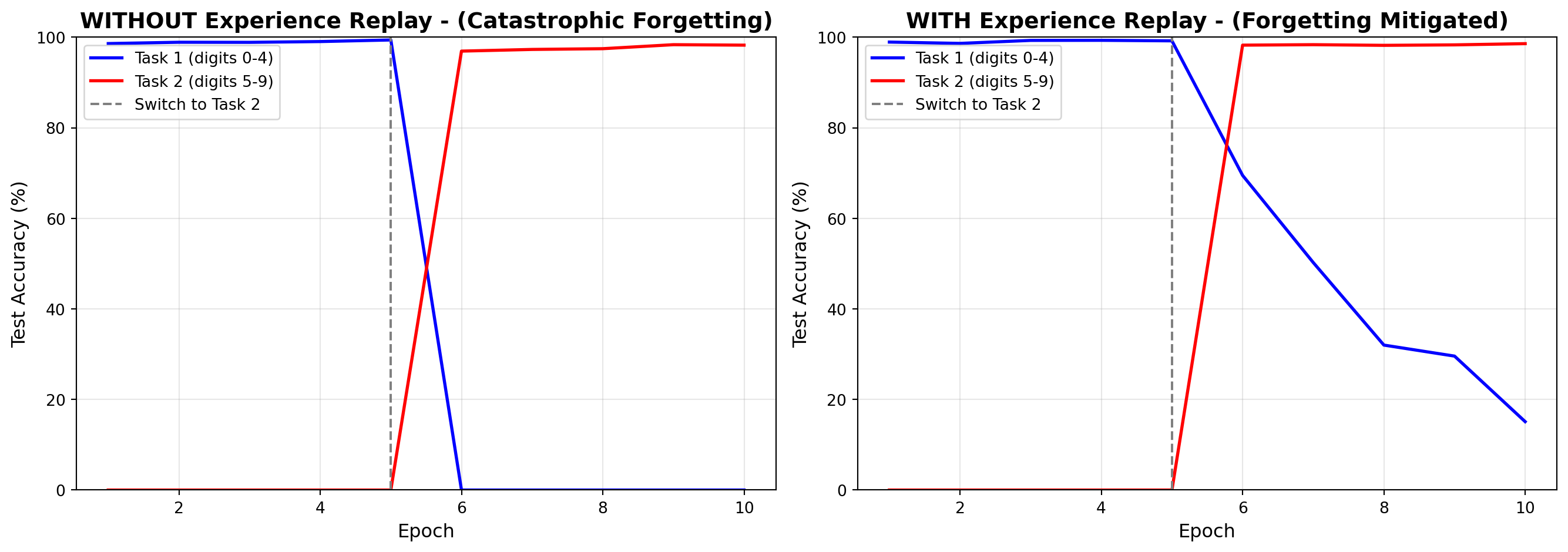
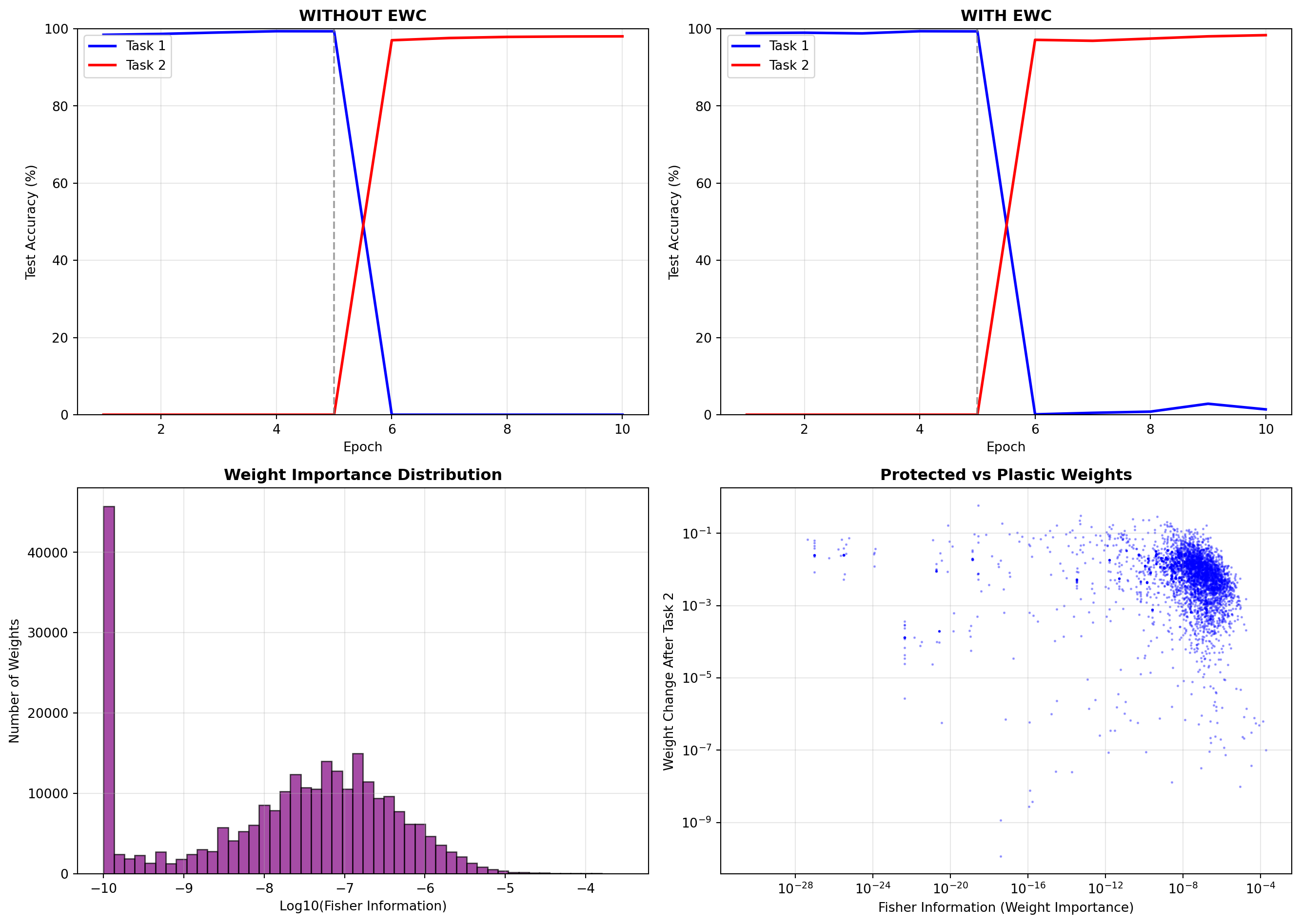

 Figure 19.5: A brain-inspired cognitive architecture featuring specialized modules (vision, language, memory, motor control) connected to a global workspace through an attentional gating mechanism. This design mimics the brain’s modular organization and enables flexible, context-aware intelligence.