24  Multimodal & Diffusion Models

NoteLearning Objectives

By the end of this chapter, you will be able to:

• Understand the principles of multimodal learning and their parallels to multisensory integration in the brain.
• Master Vision Transformer (ViT) architecture and how it enables treating images as sequences.
• Master the core concepts behind diffusion models for generative AI.
• Connect the architecture of models like CLIP and Stable Diffusion to their biological inspirations.
• Analyze how different data modalities are fused into a shared representation space using cross-attention.
• Explain the mechanisms of text-to-image generation.
• Understand speech processing (ASR/TTS) and its parallels to auditory cortex processing in the superior temporal gyrus.

24.1 16.1 Multimodal Learning: Fusing Senses

Figure 24.1: Multimodal AI systems fuse visual and linguistic representations into a shared embedding space.

The world is not experienced in a single modality. We see a dog, hear it bark, and feel its fur. The brain seamlessly fuses these streams of information into a single, coherent concept of “dog.” Multimodal learning in AI is the pursuit of this same capability: building models that can process and reason about information from multiple sources, like text, images, audio, and video.

The goal is to move beyond models that only understand text or only understand images, and towards models that have a more holistic, human-like understanding of the world.

16.1.1 Vision Transformer (ViT): Treating Images as Sequences

Before we can fuse vision and language, we need a powerful image encoder. For decades, Convolutional Neural Networks (CNNs) dominated computer vision. Then, in 2020, researchers at Google asked a radical question: What if we just use the same Transformer architecture that works so well for text?

The result was the Vision Transformer (ViT), which achieved state-of-the-art results and became the foundation for modern multimodal models like CLIP.

The Core Insight: Images as Sequences of Patches

The Transformer architecture expects a sequence of tokens. For text, this is natural: words or subwords. But what’s a “token” for an image?

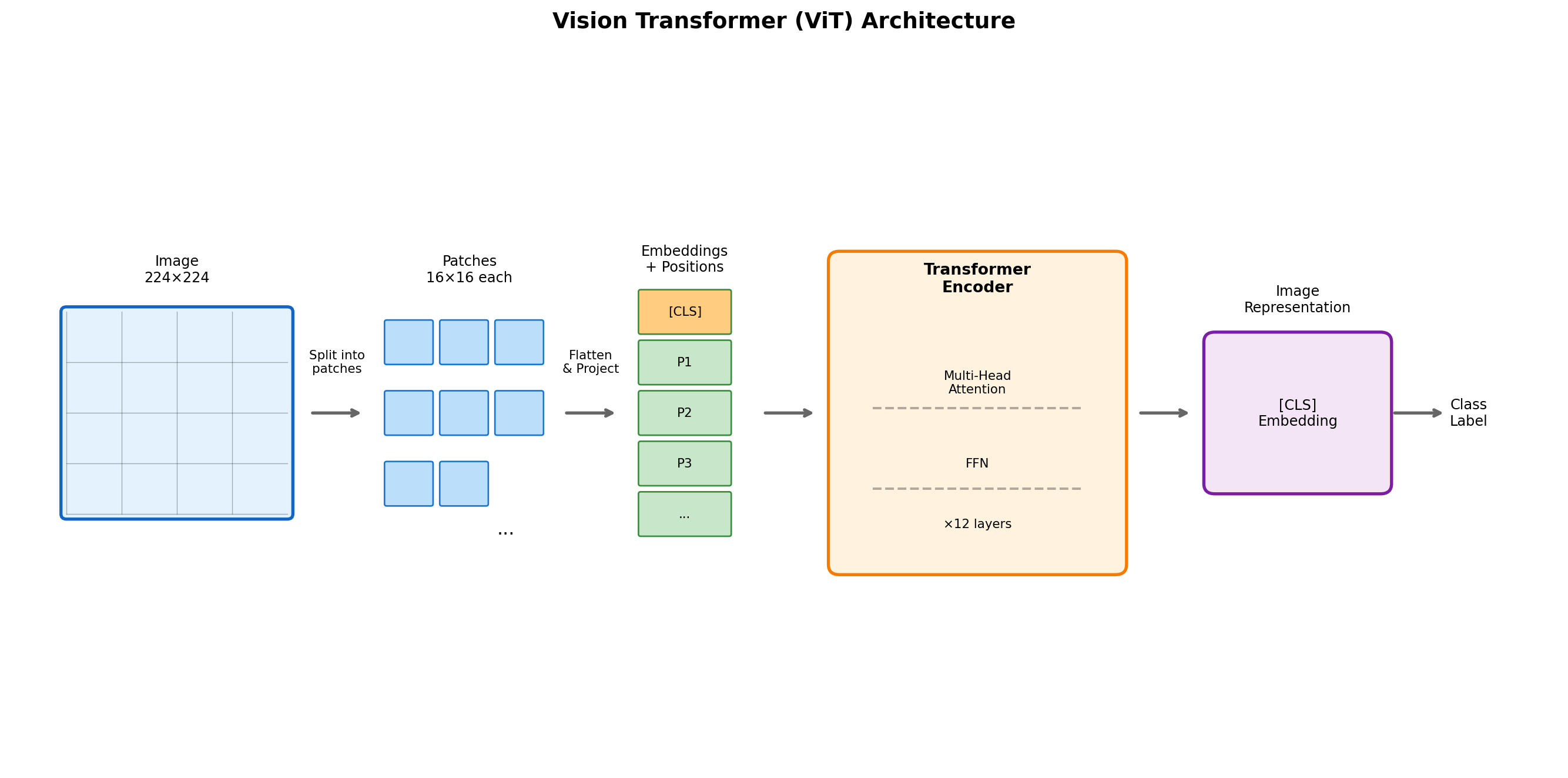
ViT’s answer: divide the image into patches.

┌─────────────────────────────────────────────────────┐
│              Original Image (224×224)               │
├───────┬───────┬───────┬───────┬───────┬───────┬─────┤
│ Patch │ Patch │ Patch │ Patch │ Patch │ Patch │ ... │
│  1    │  2    │  3    │  4    │  5    │  6    │     │
│(16×16)│(16×16)│(16×16)│(16×16)│(16×16)│(16×16)│     │
├───────┼───────┼───────┼───────┼───────┼───────┤     │
│ Patch │ Patch │ Patch │ Patch │ Patch │ Patch │     │
│  15   │  16   │  17   │  18   │  19   │  20   │     │
│       │       │       │       │       │       │     │
└───────┴───────┴───────┴───────┴───────┴───────┴─────┘
       ↓               ↓               ↓
   Flatten & Linear Projection → Sequence of Embeddings
       ↓               ↓               ↓
    [CLS] [Patch 1] [Patch 2] ... [Patch 196] → Transformer

The ViT Pipeline:

1. Patch Extraction: Split a 224×224 image into 196 patches of 16×16 pixels each
2. Linear Projection: Flatten each patch (16×16×3 = 768 values) and project to embedding dimension
3. Position Embeddings: Add learnable position embeddings (the Transformer has no built-in notion of spatial order)
4. [CLS] Token: Prepend a special classification token (like BERT)
5. Transformer Encoder: Process the sequence through standard Transformer layers
6. Classification: The [CLS] token’s final representation is used for prediction

Why Does ViT Work?

The key insight is that attention is all you need, even for images:

1. Global Receptive Field: Unlike CNNs, which build up receptive fields layer by layer, each ViT layer can attend to the entire image. The model can directly relate a patch in the corner to one in the center.

2. Fewer Inductive Biases: CNNs have built-in assumptions about images (local connectivity, translation equivariance). ViT has almost none and learns everything from data. This makes it more flexible but requires more training data.

3. Scalability: Transformers scale efficiently with compute. ViT-G (1.8B parameters) achieves near-perfect ImageNet accuracy.

4. Unification with Language: Using the same architecture for both vision and language makes fusion natural. The image and text encoders in CLIP are both Transformers, speaking the same “architectural language.”

The Data Requirement Trade-off:

ViT’s lack of inductive biases is a double-edged sword: - Small data: CNNs outperform ViT (built-in biases help) - Large data (>100M images): ViT outperforms CNNs (it learns better biases from data)

This is why ViT became dominant for large-scale pretraining (like CLIP with 400M image-text pairs) but may not be ideal for small, specialized datasets.

TipNeuroscience Connection: Receptive Fields in Visual Cortex

ViT’s architecture parallels a key debate in visual neuroscience: local vs. global processing.

The Traditional View (CNN-like): Early visual cortex (V1) processes local features through small receptive fields. Information flows hierarchically, with each layer integrating a slightly larger region, until high-level areas (inferotemporal cortex) represent entire objects. This is exactly how CNNs work.

The ViT-like Alternative: However, the brain also has long-range horizontal connections within V1 that link distant regions. And attention-based mechanisms in parietal cortex can globally modulate visual processing based on task demands.

Modern neuroscience increasingly recognizes that both local and global processing occur in parallel: - Feedforward sweep: Rapid, local, hierarchical (CNN-like) - Recurrent/feedback processing: Slower, global, context-dependent (Transformer-like)

ViT may be modeling the global, attention-based component of visual processing that complements local feature extraction. Interestingly, hybrid models (CNN + Transformer) often outperform pure ViT, just as the brain uses both mechanisms.

ViT Variants and Modern Extensions

Patch Size Trade-offs: - Smaller patches (8×8): More tokens, finer detail, higher compute - Larger patches (32×32): Fewer tokens, faster, but may miss details

Popular Variants: - DeiT (Data-efficient Image Transformer): Better training recipes, works with less data - Swin Transformer: Hierarchical ViT with shifted windows for efficiency - BEiT: BERT-style pretraining for vision (masked patch prediction) - DINO/DINOv2: Self-supervised ViT learning powerful features without labels

ViT has become the default image encoder for modern multimodal models. Understanding it is essential for understanding CLIP, Stable Diffusion, and beyond.

16.1.2 Joint Embedding Spaces and CLIP

A core technique in multimodal learning is to create a joint embedding space, a shared representational space where different modalities can be compared and combined. The breakthrough model that popularized this approach is CLIP (Contrastive Language-Image Pre-training).

CLIP was trained on a massive dataset of 400 million image-text pairs scraped from the internet. Its training objective was simple but powerful: 1. Take a batch of images and their corresponding text captions. 2. Encode all images and all text captions into vectors in a shared space. 3. The model’s goal is to make the vector for a correct image-text pair as similar as possible (high cosine similarity) while making the vectors for all incorrect pairs as dissimilar as possible.

This is a contrastive objective. By learning to match images with their descriptions, CLIP develops a rich understanding of visual concepts that is grounded in natural language. It learns that the pixels forming a picture of a cat are semantically linked to the letters forming the word “cat.”

TipNeuroscience Connection: Hebbian Learning and Cross-Modal Association

CLIP’s training process is a large-scale implementation of a principle that has long been central to neuroscience: Hebbian learning, often summarized as “neurons that fire together, wire together.”

When we see an apple and hear the word “apple” simultaneously, the neurons representing the visual features of the apple and the neurons representing the auditory features of the word are active at the same time. This co-activation strengthens the synaptic connections between them. Over time, this creates a strong cross-modal association: seeing an apple can evoke the word, and hearing the word can evoke a mental image.

CLIP’s contrastive objective achieves a similar outcome. By maximizing the similarity of co-occurring image-text pairs, it strengthens the connection between their representations in the joint embedding space, effectively wiring the visual and linguistic “neurons” together.

Figure 16.1b: Detailed CLIP architecture showing both the image encoder (Vision Transformer) and text encoder (GPT-style Transformer) pathways. Images are split into patches and processed through 12 Transformer layers, while text is tokenized and processed through a separate Transformer. Both are projected into a 512-dimensional joint embedding space where contrastive loss maximizes similarity for matched image-text pairs while minimizing similarity for mismatched pairs. This architecture enables zero-shot classification and cross-modal retrieval.

16.1.3 Multimodal Architectures

Most multimodal models consist of: - Specialized Encoders: One encoder for each modality (e.g., a Vision Transformer for images, a text Transformer for language). - A Projection Head: A small neural network that maps the output of each encoder into the shared joint embedding space. - A Fusion Mechanism: A method for combining the representations, which can be as simple as the contrastive loss or more complex, involving cross-attention layers where one modality attends to the other.

Figure 16.1: A typical multimodal architecture. Separate encoders process each modality, and their outputs are projected into a shared representation space where they can be compared and fused.

16.1.4 Cross-Attention: The Key to Multimodal Fusion

While simple concatenation or contrastive learning can combine modalities, cross-attention represents a more sophisticated fusion mechanism that allows one modality to dynamically query information from another.

Figure 16.1c: Cross-attention mechanism in multimodal models. A text query (“What animal is this?”) attends to different image patches with varying attention weights. High attention (0.75) focuses on the “dog” patch, while lower attention goes to background elements (grass, sky, tree). The output is a weighted sum of image features, allowing the model to selectively incorporate relevant visual information based on the text query. This mechanism enables flexible, context-dependent fusion of modalities.

In cross-attention: 1. Query comes from one modality (e.g., text asking “What animal is this?”) 2. Keys and Values come from another modality (e.g., image patch embeddings) 3. Attention scores are computed as the dot product of the query with each key, then passed through softmax 4. Output is a weighted sum of values, where weights are the attention scores

Mathematically: \[\text{Attention}(Q, K, V) = \text{softmax}\left(\frac{QK^T}{\sqrt{d_k}}\right)V\]

where \(Q\) is the query from one modality, and \(K, V\) are keys and values from another modality.

Biological Parallel: This mechanism mirrors how the brain’s parietal cortex integrates visual and auditory information. When you hear a sound, neurons in auditory cortex send signals to parietal association areas, which then selectively query relevant visual cortex regions to determine the sound’s source. The attention weights determine which visual features are most relevant to the auditory input.

Cross-attention is particularly powerful because it allows asymmetric information flow. One modality can ask specific questions of another, rather than treating all information equally.

24.2 16.2 Diffusion Models: Generative Art from Noise

Figure 24.2: Diffusion models progressively denoise random noise into coherent images through iterative refinement.

While models like CLIP learn to understand multimodal data, diffusion models have revolutionized the ability to generate it. These models are the engine behind most modern high-fidelity image, audio, and video generation systems like DALL-E 3, Stable Diffusion, and Midjourney.

NoteThe Sandcastle Analogy for Diffusion

Imagine building a beautiful, intricate sandcastle on the beach. This is your pristine data (a clear image). 1. The Forward Process (Erosion): The tide comes in, and waves (noise) slowly wash over your sandcastle. With each wave, a little more detail is lost. Eventually, after many waves, your sandcastle is just a smooth, formless mound of sand—indistinguishable from any other mound. This is pure noise. This process is easy and predictable. 2. The Reverse Process (Creation): Now, imagine you could film this erosion and play it in reverse. You would see the sandcastle magically re-form from the mound. This is what a diffusion model learns to do. It doesn’t just play a recording backward; it learns the rules of how to reverse the erosion. It learns, “At this stage of erosion, what small change must I make to get one step closer to the original sandcastle?”

By training on millions of examples of sandcastles eroding, the model becomes an expert sandcastle sculptor that can start from any random mound of sand (noise) and build a brand new, unique sandcastle that looks like it could have been real.

16.2.1 The Forward and Reverse Processes

• Forward Process: This is a fixed process where Gaussian noise is gradually added to an image over a series of timesteps (\(t\)). At each step, the image becomes slightly noisier, until eventually, at the final timestep \(T\), it is pure, unstructured noise.
• Reverse Process: This is the learned process. The model, typically a U-Net architecture, is trained to predict the noise that was added at a given timestep \(t\). By subtracting this predicted noise, it can take a noisy image \(x_t\) and produce a slightly less noisy image \(x_{t-1}\).

Figure 16.2: The diffusion process. During the forward pass, noise is incrementally added to an image. The model learns the reverse process: to start with noise and incrementally denoise it to generate a clean image.

16.2.2 The U-Net and Time Conditioning

The workhorse of a diffusion model is a U-Net, a deep neural network with a symmetric encoder-decoder structure and “skip connections” that allow information to flow from the encoder to the decoder. This architecture is excellent at processing images and preserving fine-grained detail.

Crucially, the U-Net is time-conditioned. It takes two inputs: the noisy image \(x_t\) and the current timestep \(t\). This allows the model to learn different denoising strategies for different levels of noise (e.g., at high \(t\), it learns to find large-scale structures; at low \(t\), it learns to fill in fine details).

24.3 16.3 Text-to-Image Models: The Fusion of Understanding and Generation

Text-to-image models like Stable Diffusion are a brilliant synthesis of the two concepts we’ve discussed: they combine a CLIP-like text encoder for understanding with a diffusion model for generation.

Figure 16.3: The architecture of a text-to-image latent diffusion model. A text encoder creates an embedding of the prompt, which is fed into the U-Net via cross-attention at each step of the reverse diffusion process in a compressed latent space.

16.3.1 Latent Diffusion: Efficiency Through Compression

To make the process computationally feasible, models like Stable Diffusion don’t operate on the images directly. Instead, they use a Variational Autoencoder (VAE) to compress a high-resolution image into a much smaller latent space. The entire diffusion process happens in this compressed space, and the final denoised latent is then decoded back into a full-resolution image by the VAE. This is why it’s called a Latent Diffusion Model.

Figure 16.3b: Complete architecture of a latent diffusion model (Stable Diffusion). The text prompt is encoded by CLIP’s text encoder. A VAE compresses the image from 512×512×3 (786K pixels) to 64×64×4 (16K latents), a 49× reduction. The U-Net denoising network operates in this compressed latent space over 50 iterative steps, guided by text conditioning via cross-attention. Finally, the VAE decoder transforms the denoised latent back to full resolution. This architecture achieves high-quality generation at a fraction of the computational cost of pixel-space diffusion.

The Computational Advantage: - Pixel-space diffusion: Would require denoising 512×512×3 = 786,432 values at each step - Latent diffusion: Only denoises 64×64×4 = 16,384 values (49× fewer) - Result: Same visual quality, but training and inference are dramatically faster and cheaper

This is conceptually similar to how the brain doesn’t store every pixel of what you see, but rather a compressed, abstract representation. When you close your eyes and imagine an apple, you’re not reconstructing every photoreceptor activation. You’re working with a compressed “latent” representation in visual cortex.

16.3.2 Text Conditioning via Cross-Attention

This is where the magic happens. The text prompt is first encoded into a set of vectors by a text encoder (often the text encoder from CLIP). Then, at each step of the reverse diffusion process, these text vectors are fed into the U-Net using cross-attention layers.

In these layers, the noisy image representation (the Query) “attends to” the text embedding (the Key and Value). This allows the U-Net to use the information from the prompt to guide the denoising process. For example, if the prompt is “a red apple,” the cross-attention mechanism will guide the U-Net to denoise the latent in a way that forms the shape of an apple and fills it with the color red.

16.3.3 Classifier-Free Guidance: Controlling Generation Strength

To improve the adherence to the prompt, a technique called Classifier-Free Guidance is used. During generation, the model computes two noise predictions: one conditioned on the text prompt, and one unconditioned (a generic image). The final prediction is then pushed further in the direction of the conditioned prediction. This is controlled by a guidance scale parameter, which acts like a knob for how strongly the model should follow the prompt.

Figure 16.3c: Classifier-free guidance controls the trade-off between prompt adherence and generation quality. With low guidance (w=1.0), the output is generic and less detailed. With optimal guidance (w=7.5), the image is detailed and well-aligned with the prompt. With excessive guidance (w=20), the image becomes oversaturated with artifacts. The formula ε̃ = ε_uncond + w·(ε_cond - ε_uncond) amplifies the difference between conditional and unconditional predictions, pushing generation toward features emphasized in the prompt.

The Mathematics of Guidance:

The final noise prediction is computed as: \[\tilde{\epsilon} = \epsilon_{\text{uncond}} + w \cdot (\epsilon_{\text{cond}} - \epsilon_{\text{uncond}})\]

where: - \(\epsilon_{\text{uncond}}\) = noise prediction without the text prompt (creative but unfocused) - \(\epsilon_{\text{cond}}\) = noise prediction with the text prompt (prompt-aligned) - \(w\) = guidance scale (typically 5-10 for balanced results)

Interpretation: When \(w=1\), you get the conditioned prediction alone. As \(w\) increases, you move further in the direction away from the unconditional baseline toward the conditioned prediction. This amplifies the features that the prompt emphasizes while suppressing generic features.

Practical Implications: - Low guidance (w < 3): More creative, diverse outputs but weaker prompt following - Medium guidance (w = 7-8): Sweet spot with good prompt adherence and natural-looking images - High guidance (w > 15): Very literal prompt following but oversaturated, unnatural images

This parallels how our own imagination works: we can choose to strictly adhere to a mental specification (“imagine exactly what I describe”) or let our mind wander creatively (“imagine something inspired by this”).

24.4 16.4 Speech and Audio: The Auditory Modality

Speech is perhaps the most natural interface between humans and machines. Unlike text, speech is a continuous signal that unfolds in time, requiring specialized processing pipelines. This section explores how AI systems process and generate speech, drawing deep parallels to the brain’s auditory system.

16.4.1 The Speech Signal: From Sound Waves to Meaning

Speech is a remarkably complex signal. A single second of audio at CD quality (44.1 kHz) contains 44,100 samples, far more data points than a sentence of text. Yet the human brain extracts meaning from this stream effortlessly, segmenting continuous sound into phonemes, syllables, words, and sentences.

The Auditory Processing Pipeline: 1. Cochlea: Decomposes sound into frequency bands (like a biological spectrogram) 2. Auditory nerve: Encodes timing and intensity information 3. Auditory cortex: Extracts phonetic features 4. Superior temporal gyrus: Processes words and sentences 5. Wernicke’s area: Comprehends meaning

Modern speech AI follows a remarkably similar pipeline, converting raw waveforms to spectrograms to learned representations to meaning.

16.4.2 Automatic Speech Recognition (ASR)

Automatic Speech Recognition converts spoken language to text. Modern ASR systems have achieved near-human accuracy on many benchmarks, enabling voice assistants, transcription services, and accessibility tools.

The ASR Pipeline

Feature Extraction: - Mel-frequency spectrograms: Transform raw audio into time-frequency representations that match human auditory perception - Mel filter banks: Mimic the cochlea’s frequency response (logarithmic scaling, ~80 filters) - MFCC (Mel-Frequency Cepstral Coefficients): Classical features that compress spectral information

Encoder-Decoder Architecture: Modern ASR uses the same encoder-decoder Transformer architecture as machine translation: - Encoder: Processes the audio spectrogram, often with initial convolutional layers to downsample - Decoder: Autoregressively generates text tokens - Attention: Learns alignment between audio frames and text tokens

Key Models: - Whisper (OpenAI): Trained on 680,000 hours of multilingual audio, achieving robust performance across accents, noise levels, and languages - Wav2Vec 2.0 (Meta): Self-supervised pretraining on unlabeled audio, then fine-tuning with limited transcribed data - Conformer: Combines convolution (for local patterns) with Transformer attention (for global context)

TipNeuroscience Connection: Temporal Processing in the Superior Temporal Gyrus

The brain’s superior temporal gyrus (STG) is the hub for speech processing, and its neural mechanisms offer insights for AI design.

Hierarchical Temporal Processing: The STG processes speech at multiple timescales simultaneously: - Primary auditory cortex (A1): Encodes rapid acoustic features (~20-50ms windows) - Posterior STG: Processes phonemes (~50-100ms) - Anterior STG: Integrates syllables and words (~100-500ms) - Superior temporal sulcus: Processes sentences and discourse (>500ms)

This hierarchical structure is mirrored in modern ASR architectures, where: - Early convolutional layers capture fine-grained acoustic patterns - Transformer layers integrate increasingly long-range context - Final layers produce word and sentence-level representations

Predictive Coding in Auditory Cortex: Just as language models predict the next token, auditory cortex predicts upcoming sounds. When expectations are violated (unexpected phoneme, foreign accent), the brain generates a mismatch negativity (MMN) response, a neural prediction error signal. ASR systems trained with Connectionist Temporal Classification (CTC) learn similar probabilistic predictions over time.

Robustness Through Redundancy: Human speech perception is remarkably robust to noise, accents, and distortions. This is achieved through: - Multiple redundant cues (voicing, formant transitions, coarticulation) - Top-down predictions filling in missing information - Integration across time windows

Modern robust ASR achieves similar robustness through data augmentation, self-supervised pretraining, and attention over long contexts.

16.4.3 Text-to-Speech (TTS) and Speech Synthesis

Text-to-Speech systems convert written text to natural-sounding speech. Modern TTS has achieved remarkable quality, enabling everything from voice assistants to audiobook narration.

The TTS Pipeline

Text Analysis: - Text normalization: “Dr.” → “Doctor”, “$100” → “one hundred dollars” - Grapheme-to-phoneme (G2P): Convert text to phonetic representation - Prosody prediction: Determine pitch, duration, and stress patterns

Acoustic Modeling: Modern TTS uses neural vocoders to generate high-fidelity audio: - Tacotron 2: Sequence-to-sequence model generating mel spectrograms - WaveNet/WaveGlow: Neural vocoders converting spectrograms to waveforms - VITS: End-to-end TTS with variational inference for expressive synthesis

Neural Codec Language Models: The New Paradigm

The latest generation of speech models treats audio as a sequence of discrete tokens, just like text:

1. Audio Codec: A neural network compresses audio to discrete tokens (e.g., EnCodec, SoundStream)
2. Language Model: A Transformer predicts audio tokens conditioned on text
3. Decoder: Converts tokens back to waveforms

VALL-E pioneered this approach: - Encodes 3 seconds of reference speech as a prompt - Generates new speech in the same voice for any text - Enables zero-shot voice cloning

This tokenized approach unifies speech with text in a single multimodal language model, enabling models like GPT-4o to handle both modalities natively.

16.4.4 Video Generation and Temporal Consistency

Video extends image generation to the temporal dimension, adding significant complexity:

Challenges: - Temporal consistency: Objects must persist and move coherently - Motion dynamics: Physical plausibility of movement - Computational cost: Each frame requires full generation - Long-range coherence: Scenes must remain consistent across many seconds

Approaches: - 3D U-Nets: Process video as 3D tensors (height × width × time) - Temporal attention: Attention across frames for consistency - Keyframe interpolation: Generate key frames, fill in between - Autoregressive generation: Generate frame-by-frame, conditioning on history

Notable Models: - Sora (OpenAI): Generates minute-long videos with remarkable consistency - Runway Gen-3: Commercial video generation platform - Make-A-Video (Meta): Text-to-video with temporal U-Nets

TipNeuroscience Connection: Motion Processing in MT/V5

The brain has a dedicated area for motion processing: area MT (middle temporal), also called V5. Neurons here are selective for motion direction and speed, integrating information across space and time.

Key properties relevant to video AI: - Direction selectivity: Neurons fire for specific motion directions, similar to how video models learn motion patterns - Optic flow processing: MT computes global motion patterns, analogous to optical flow estimation in video models - Prediction and interpolation: The brain interpolates between discrete visual samples (at ~10-15 Hz consciously perceived) to create smooth motion, similar to frame interpolation in video generation

The brain’s ability to perceive smooth motion from discrete samples inspired the use of temporal interpolation in video generation pipelines.

24.5 16.5 Real-World Applications: Where Multimodal AI Makes Impact

While text-to-image generation captures public imagination, multimodal AI has profound applications across science, medicine, and accessibility.

16.5.1 Medical Diagnosis: Combining Imaging and Clinical Data

Modern medicine generates data from multiple sources: medical images (MRI, CT, X-ray), clinical notes, lab results, genetic data, and patient history. Multimodal AI models can integrate these disparate sources to achieve diagnostic accuracy exceeding single-modality approaches.

Figure 16.5: Medical multimodal AI for brain tumor diagnosis. The system integrates three modalities: (1) MRI scans processed by a 3D CNN to extract visual features, (2) clinical notes processed by BERT to extract textual features, (3) structured data (age, sex, history, labs) processed by an MLP. A multimodal fusion layer combines these representations using cross-attention and concatenation. The classification head predicts tumor type and grade. This fusion of imaging, text, and structured data achieves higher accuracy than any single modality alone by capturing complementary information.

Case Study: Brain Tumor Classification

A 2021 study demonstrated that combining MRI scans with clinical notes improved glioblastoma detection from 87% accuracy (imaging alone) to 94% accuracy (multimodal). The multimodal model learned that certain textual patterns (“progressive headaches,” “new-onset seizures”) combined with specific imaging features (irregular enhancement, perilesional edema) strongly predicted high-grade tumors. This was a pattern neither modality revealed independently.

Key Advantages: - Complementary Information: Imaging shows anatomy; text describes symptoms and progression - Handling Missing Data: If one modality is unavailable, the model can still make predictions using available modalities - Explainability: Cross-attention weights reveal which image regions and which text phrases contributed to the diagnosis

16.5.2 Scientific Discovery: Protein Structure and Function

Multimodal AI has accelerated biological discovery by integrating protein sequence data (1D text-like information) with 3D structural data (spatial information) and functional annotations (text descriptions).

AlphaFold 2 combines sequence information with multiple sequence alignments and structural templates to predict 3D protein structure. More recent work integrates this with: - Textual descriptions of protein function from literature - Gene expression data showing when and where proteins are active - Interaction networks showing which proteins work together

This multimodal integration enables: - Predicting protein function from structure alone - Designing novel proteins with desired properties - Understanding disease mutations by seeing how they affect both structure and function

16.5.3 Accessibility: Multimodal Assistive Technologies

Multimodal AI enables powerful accessibility tools:

Image Captioning for Blind Users: Models like CLIP can generate detailed descriptions of images, enabling blind users to access visual content on the web. Advanced systems can answer questions about images (“What color is the shirt?”, “Is there a ramp?”).

Sign Language Translation: Multimodal models that process hand gestures (video), facial expressions (vision), and body posture (pose estimation) can translate sign language to text/speech and vice versa, breaking communication barriers for deaf individuals.

Augmentative Communication for ALS: Brain-computer interfaces combined with language models enable patients with locked-in syndrome to communicate by: 1. Neural signals decoded from motor cortex → intended letter/word 2. Language model provides text predictions 3. Text-to-speech generates audio output

This is a profoundly multimodal pipeline: neural → linguistic → auditory.

16.5.4 Creative Applications and Implications

Text-to-image, text-to-video, and text-to-music models have democratized creative expression, enabling anyone to generate professional-quality content from descriptions. However, this raises important questions:

Positive Impacts: - Accessibility for people without traditional artistic skills - Rapid prototyping for designers and filmmakers - Educational visualization of historical events or scientific concepts

Challenges: - Copyright and attribution (models trained on copyrighted work) - Job displacement for human artists - Misinformation and deepfakes - Bias amplification (models perpetuate biases in training data)

The responsible development and deployment of multimodal generative AI requires ongoing dialogue between technologists, artists, ethicists, and policymakers.

24.6 16.6 Training Challenges and Solutions

Building effective multimodal models presents unique challenges beyond single-modality systems.

16.6.1 Modality Imbalance

Different modalities learn at different rates. In an image-text model: - Visual features often learn quickly (edges, textures apparent in early training) - Linguistic features may require more examples to capture semantics

Solution: Use modality-specific learning rates, with slower rates for the faster-learning modality. Alternatively, use gradient balancing techniques that ensure neither modality dominates the optimization.

16.6.2 Alignment Across Modalities

Real-world data is often noisily aligned. Image-text pairs scraped from the internet may have: - Weak alignment: Caption describes overall scene but misses details - Misalignment: Caption doesn’t match the image at all - Ambiguity: Multiple valid captions for one image

Solution: - Use contrastive learning (like CLIP) which is robust to some noise - Filter training data using pre-trained alignment models - Use hard negative mining to focus learning on difficult cases

16.6.3 Computational Costs

Training models like CLIP or Stable Diffusion requires: - Massive datasets: 400M+ image-text pairs for CLIP - Large compute: Thousands of GPU-hours - Memory: Billions of parameters

Solutions: - Latent diffusion reduces compute by 49× compared to pixel-space diffusion - Efficient architectures: Use lightweight encoders for some modalities - Progressive training: Start with low-resolution, gradually increase - Knowledge distillation: Train a large teacher model, then compress to a smaller student

16.6.4 Evaluation Challenges

How do you measure if a generated image is “good”? Unlike classification (clear accuracy metric), generative models require multi-faceted evaluation:

Automated Metrics: - FID (Fréchet Inception Distance): Measures distribution similarity - CLIP Score: Measures image-text alignment - Inception Score: Measures diversity and quality

Human Evaluation: - Prompt adherence: Does the image match the description? - Photorealism: Does it look like a real photo? - Artifacts: Are there visual glitches or distortions?

Ethical Evaluation: - Bias audit: Does the model perpetuate stereotypes? - Safety: Can it generate harmful content?

Comprehensive evaluation requires all three categories.

24.7 16.7 Neural Multimodal Integration: Lessons from the Brain

The brain’s ability to integrate sensory information is a key inspiration for multimodal AI.

16.7.1 Multisensory Integration in the Brain

The brain does not process senses in isolation. Information from different sensory organs converges in multisensory association areas, such as the superior colliculus, superior temporal sulcus (STS), and parietal cortex. In these regions, neurons exist that respond to stimuli from multiple modalities. For example, a neuron in the STS might fire in response to both the sight of a face and the sound of the corresponding voice.

This integration is not just a simple summation; it is a sophisticated process where one modality can influence the perception of another. The brain implements principles remarkably similar to cross-attention: - Selective integration: Not all inputs are weighted equally; context determines which modality dominates - Temporal synchrony: Inputs arriving within ~200ms are bound together as belonging to the same event - Spatial coincidence: Visual and auditory inputs from the same location are more strongly integrated

16.7.2 Cross-Modal Illusions: When Senses Collide

The power of the brain’s multisensory fusion is most apparent when it’s “tricked” by cross-modal illusions. - The McGurk Effect: A famous illusion where seeing a person’s lips form the sound “ga” while hearing the sound “ba” results in the perception of a third sound, “da.” This shows that the visual information is overriding and altering the auditory perception. - The Ventriloquist Effect: The brain assumes that a sound is coming from a plausible visual source, even if it isn’t. This is why a ventriloquist’s voice seems to come from the dummy’s mouth.

These illusions reveal that perception is not a passive reception of sensory data but an active process of inference and integration. The brain makes a “best guess” about the state of the world by combining all available evidence. This is conceptually similar to how a multimodal AI model fuses representations to arrive at a unified understanding.

This section would contain a hands-on implementation of a simple diffusion model.

True

ImportantChapter Summary

In this chapter, we explored the fusion of perception and generation in modern AI, drawing strong parallels to the brain’s own multimodal capabilities.

• Multimodal Learning aims to build models that, like the brain, can integrate information from multiple senses. Techniques like CLIP use contrastive learning to create a joint embedding space where text and images can be compared, mirroring the brain’s cross-modal associations.
• Diffusion Models have revolutionized generative AI. By learning to reverse a process of gradually adding noise, they can generate stunningly realistic and novel data. This two-step process of erosion and creation provides a powerful and stable method for generation.
• Text-to-Image Models like Stable Diffusion represent the pinnacle of multimodal generation. They combine a text encoder (for understanding) with a latent diffusion model (for generation), using cross-attention to guide the image creation process based on a text prompt.
• Speech and Audio Processing bridges the gap between continuous acoustic signals and discrete language, with modern ASR and TTS systems achieving near-human performance. The brain’s hierarchical temporal processing in the superior temporal gyrus provides insights for building robust, real-time speech systems.
• The brain’s multisensory integration in regions like the superior temporal sulcus provides a biological blueprint for these systems. Cross-modal illusions like the McGurk effect reveal the deep, inferential nature of perception, a principle that is increasingly being built into our AI models.

ImportantKnowledge Connections

Looking Back - Chapter 11 (Sequence Models): The Transformer architecture, which is the backbone of the text encoders used in models like CLIP and Stable Diffusion, was covered in detail. - Chapter 12 (LLMs): The principles of large-scale pre-training and representation learning from LLMs are directly applied to the language component of these multimodal systems.

Looking Forward - Chapter 14 (Bridging Bio & AI): The concepts of multimodal integration and generative models are central to building more brain-like AI architectures. - Chapter 19 (Cognitive Neuroscience & DL): We will revisit how these generative models can be used not just to create art, but also as scientific tools to model and understand brain function.

24.8 Exercises

Conceptual Questions

1. CLIP and Hebbian Learning: The chapter connects CLIP’s contrastive learning to Hebbian learning (“neurons that fire together, wire together”). Explain this connection in detail. How is maximizing the similarity of co-occurring image-text pairs analogous to synaptic strengthening through correlated activity? What role does the contrastive part (pushing apart non-matching pairs) play, and does the brain implement a similar mechanism?

2. The McGurk Effect and Cross-Modal Attention: The McGurk effect demonstrates that visual information can override auditory perception in speech processing. How might cross-attention mechanisms in multimodal AI models relate to this phenomenon? Design a computational model (in words, not code) that could produce McGurk-like effects using cross-attention between audio and visual modalities.

3. Diffusion as an Iterative Refinement Process: Diffusion models progressively denoise an image over many steps, moving from coarse structure to fine detail. Compare this to artistic and cognitive processes of creation. How do human artists work (e.g., sketch to refinement)? How might the brain generate mental imagery? What computational advantages might an iterative process have over a single-step generation?

4. Joint Embedding Spaces and Concepts: CLIP creates a shared representation space where “cat” (text) and a photo of a cat are nearby vectors. Discuss what this means for the model’s “understanding” of concepts. Does CLIP truly understand what a cat is, or is it just performing sophisticated pattern matching? How does this relate to debates about symbol grounding and meaning in cognitive science?

Computational Problems

5. Building a Mini-CLIP Model: Implement a simplified version of CLIP using a small dataset:
   • Collect or use an existing dataset of image-text pairs (e.g., 1,000 images from a few categories with simple captions)
   • Implement separate encoders for images (e.g., a small CNN or Vision Transformer) and text (e.g., a simple Transformer or bag-of-words with an MLP)
   • Implement the contrastive loss function
   • Train the model and visualize the learned embedding space (use t-SNE or UMAP)
   • Test zero-shot classification: can the model classify images into novel categories just from text descriptions?
   • Analyze failure cases: what kinds of mismatches does the model make?
6. Implementing a Simple Diffusion Model: Build a diffusion model from scratch for a simple dataset (e.g., MNIST or 2D toy data):
   • Implement the forward process (adding Gaussian noise over T timesteps)
   • Build a U-Net or simple denoising network that takes the noisy image and timestep as input
   • Train the model to predict the noise at each timestep
   • Implement the reverse process to generate new samples
   • Visualize the denoising trajectory for several examples
   • Experiment with different numbers of diffusion steps and analyze the trade-off between quality and computation
7. Text-Conditioned Generation: Extend your diffusion model (or use a pre-trained one like Stable Diffusion via APIs) to be text-conditioned:
   • Implement or use a text encoder to create embeddings
   • Add cross-attention layers to condition the denoising process on text
   • Generate images from various prompts and analyze the results
   • Experiment with classifier-free guidance strength: how does it affect prompt adherence vs. image quality?
   • Create “adversarial prompts” that reveal the model’s biases or limitations
8. Analyzing Multimodal Representations: Using a pre-trained CLIP model:
   • Extract embeddings for a diverse set of images and text descriptions
   • Analyze the geometry of the joint embedding space (e.g., measure distances, find nearest neighbors)
   • Test compositional understanding: does “red car” embed closer to “red truck” or “blue car”?
   • Probe for biases: how are concepts related to gender, race, or profession clustered?
   • Construct “analogies” in embedding space (e.g., “king - man + woman = ?” in text, applied to images)

Discussion Questions

9. Multimodal AI and Grounded Cognition: In embodied cognition theory, abstract concepts are grounded in sensorimotor experience (e.g., understanding “cat” involves visual, tactile, and auditory memories). Discuss how multimodal AI models like CLIP relate to this theory:
   • Do models trained on image-text pairs have “grounded” representations compared to text-only LLMs?
   • What sensorimotor modalities are still missing from current AI (e.g., touch, proprioception, taste)?
   • How might incorporating additional modalities (audio, video, 3D, robotics) lead to more robust and general AI?
   • Could a fully multimodal AI system develop something resembling true understanding?
10. Ethical Implications of Generative Models: Diffusion models can create photorealistic fake images, videos, and audio. Discuss the societal implications:

• What are the risks (e.g., deepfakes, misinformation, copyright issues, job displacement for artists)?
• What are the benefits (e.g., accessibility for creative expression, scientific visualization, data augmentation)?
• How do we balance innovation with responsibility? Should there be regulations, watermarking requirements, or usage restrictions?
• From a neuroscience perspective, how might the prevalence of AI-generated content affect human perception, trust, and cognitive processing of visual information?
• What technical solutions (e.g., detection tools, provenance tracking) and social solutions (e.g., media literacy education) are needed?

24.9 References

Dhariwal, P., & Nichol, A. (2021). Diffusion models beat GANs on image synthesis. Advances in Neural Information Processing Systems, 34, 8780-8794. https://arxiv.org/abs/2105.05233

Driver, J., & Noesselt, T. (2008). Multisensory interplay reveals crossmodal influences on ‘sensory-specific’ brain regions, neural responses, and judgments. Neuron, 57(1), 11-23. https://doi.org/10.1016/j.neuron.2007.12.013

Ghahramani, Z., Wolpert, D. M., & Jordan, M. I. (1997). Computational models of sensorimotor integration. In P. G. Morasso & V. Sanguineti (Eds.), Self-organization, computational maps, and motor control (pp. 117-147). Elsevier.

Ho, J., Jain, A., & Abbeel, P. (2020). Denoising diffusion probabilistic models. Advances in Neural Information Processing Systems, 33, 6840-6851. https://arxiv.org/abs/2006.11239

McGurk, H., & MacDonald, J. (1976). Hearing lips and seeing voices. Nature, 264(5588), 746-748. https://doi.org/10.1038/264746a0

Radford, A., Kim, J. W., Hallacy, C., Ramesh, A., Goh, G., Agarwal, S., Sastry, G., Askell, A., Mishkin, P., Clark, J., Krueger, G., & Sutskever, I. (2021). Learning transferable visual models from natural language supervision. International Conference on Machine Learning. https://arxiv.org/abs/2103.00020

Ramesh, A., Dhariwal, P., Nichol, A., Chu, C., & Chen, M. (2022). Hierarchical text-conditional image generation with CLIP latents. arXiv preprint arXiv:2204.06125. https://arxiv.org/abs/2204.06125

Rombach, R., Blattmann, A., Lorenz, D., Esser, P., & Ommer, B. (2022). High-resolution image synthesis with latent diffusion models. IEEE Conference on Computer Vision and Pattern Recognition. https://arxiv.org/abs/2112.10752

Saharia, C., Chan, W., Saxena, S., Li, L., Whang, J., Denton, E., Ghasemipour, S. K. S., Ayan, B. K., Mahdavi, S. S., Lopes, R. G., Salimans, T., Ho, J., Fleet, D. J., & Norouzi, M. (2022). Photorealistic text-to-image diffusion models with deep language understanding. Advances in Neural Information Processing Systems, 35. https://arxiv.org/abs/2205.11487

Shams, L., & Kim, R. (2010). Crossmodal influences on visual perception. Physics of Life Reviews, 7(3), 269-284. https://doi.org/10.1016/j.plrev.2010.04.006

Sohl-Dickstein, J., Weiss, E., Maheswaranathan, N., & Ganguli, S. (2015). Deep unsupervised learning using nonequilibrium thermodynamics. International Conference on Machine Learning. https://arxiv.org/abs/1503.03585

Stein, B. E., & Stanford, T. R. (2008). Multisensory integration: Current issues from the perspective of the single neuron. Nature Reviews Neuroscience, 9(4), 255-266. https://doi.org/10.1038/nrn2331