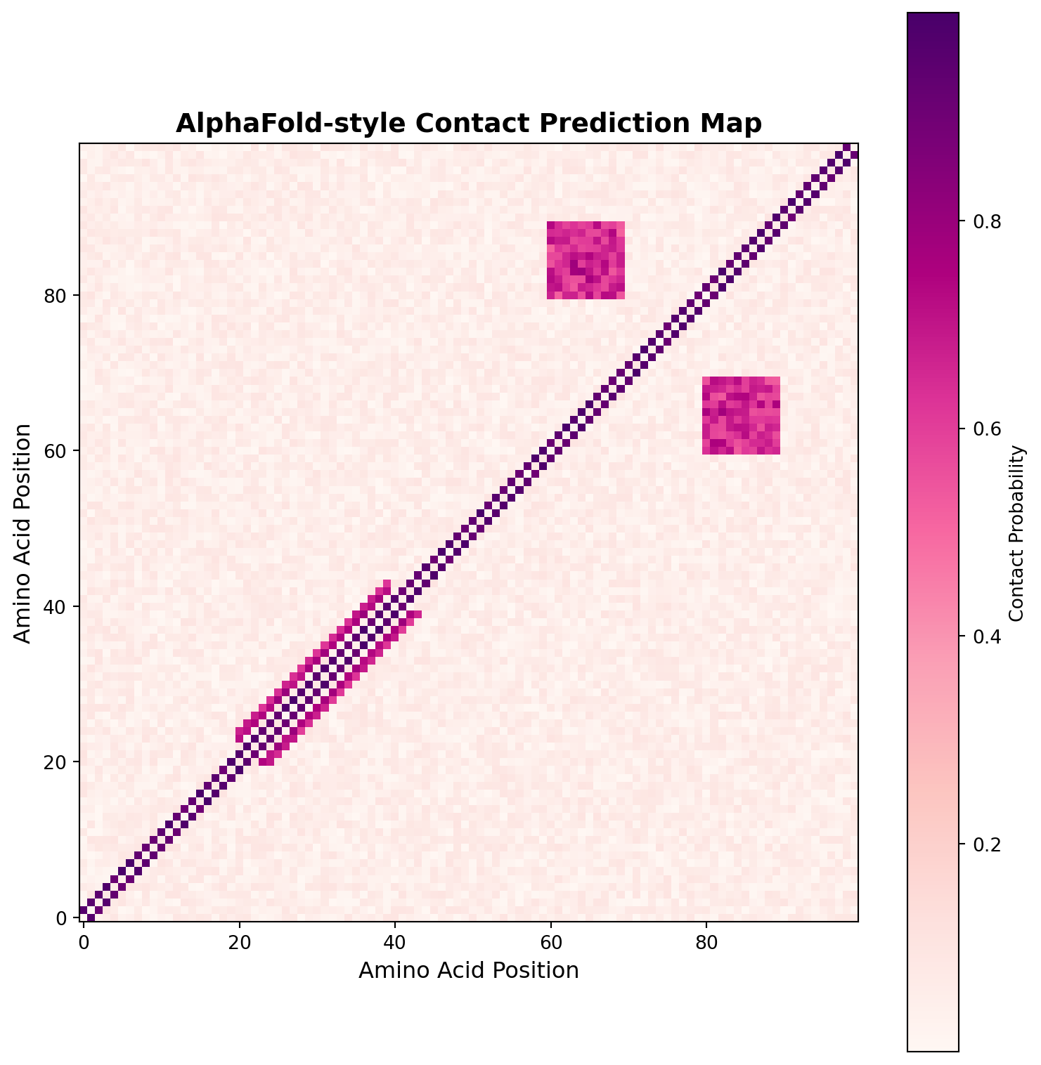
Contact map shows predicted spatial proximity between amino acids
Diagonal: Sequential contacts | Patterns: Secondary structures (helices, sheets)Learning Objectives By the end of this chapter, you will be able to:
- Understand the revolutionary role of AI as a new kind of scientific instrument for neuroscience.
- Explain how AI is used to decode thoughts, map connections, and discover the underlying structure of neural activity.
- Analyze how deep learning models can find meaningful patterns in high-dimensional neural data.
- Appreciate the clinical impact of these tools in diagnosing and treating neurological disorders.
- Envision how AI-driven discovery will continue to accelerate our understanding of the brain.
For centuries, our tools for understanding the brain were limited. We could study its anatomy, record the electrical crackle of a single neuron, or see the slow ebb and flow of blood in an fMRI scanner. But we struggled to understand the language of the brain’s vast, high-dimensional neural populations. We were missing the right kind of microscope.
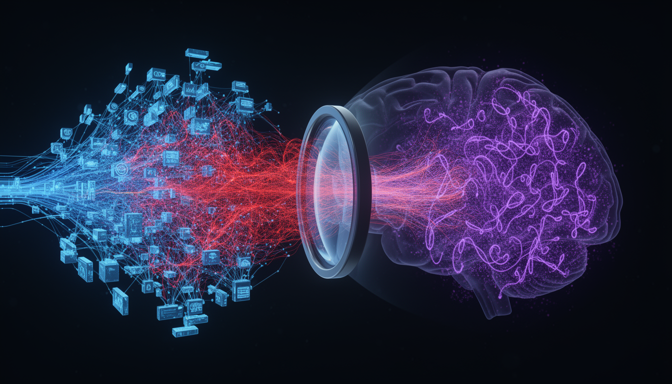
Artificial intelligence, particularly deep learning, has given us that microscope. It is a computational microscope that allows us to look into the complex activity of thousands of neurons and see the hidden patterns, structures, and dynamics that underlie cognition. This is the other half of the virtuous cycle of NeuroAI: AI is not just inspired by the brain; it is becoming our most powerful tool for understanding it.
This chapter explores the functions of this new microscope, showing how it allows us to: 1. See the Unseen: Decode thoughts and percepts directly from neural activity. 2. Find the Structure: Discover the low-dimensional “shape” of neural computations. 3. Map the Connections: Automate the reconstruction of the brain’s wiring diagram. 4. Simulate the System: Build and test large-scale models of brain circuits.
The most dramatic application of our computational microscope is neural decoding: translating the raw electrical activity of the brain into its meaningful content.
Every thought, perception, and movement is encoded in the coordinated firing of millions of neurons. This “neural code” is incredibly complex, high-dimensional, and noisy. A person’s intent to say a word is not represented by a single neuron firing, but by a fleeting, intricate pattern of activity across a vast population. Traditional statistical methods struggled to find the signal in this noise.
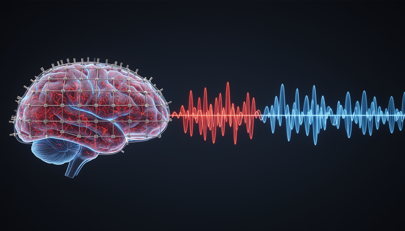
Deep learning models, especially those designed for sequences like LSTMs and Transformers, are perfectly suited for this task. Researchers can record neural activity (e.g., using ECoG grids on the surface of the brain) while a person speaks or listens to speech. A deep learning model is then trained to learn the mapping between the complex spatio-temporal patterns of neural data and the corresponding words.
The results have been breathtaking. Recent studies have shown that these AI decoders can: - Reconstruct speech with remarkable clarity directly from brain activity. - Reconstruct visual scenes, including faces, that a person is looking at from fMRI data. - Decode motor intent in people with paralysis, allowing them to control robotic limbs or type on a screen.
This is the computational microscope in action, making the invisible patterns of thought visible and usable.
The clinical implications of neural decoding are profound. For patients with locked-in syndrome or paralysis from ALS or stroke, AI-powered BCIs are restoring the ability to communicate. By decoding the neural signals associated with intended speech, these systems can drive a speech synthesizer, giving a voice back to those who have lost it.
While neural decoding operates at the systems level, AI is also revolutionizing our understanding of the brain’s molecular machinery. One of the most dramatic examples is AlphaFold, DeepMind’s deep learning system for predicting protein structure from amino acid sequences.
For decades, determining the three-dimensional structure of proteins was one of biology’s grand challenges. Traditional methods like X-ray crystallography and cryo-electron microscopy are expensive, time-consuming, and often fail for membrane proteins, the very proteins that form the ion channels and receptors essential for neural function.
The challenge is that a protein’s function is entirely determined by its 3D shape, but that shape is determined by the complex folding of a linear chain of amino acids. The number of possible configurations is astronomically large, making brute-force simulation infeasible.
AlphaFold 2, released in 2020, uses a sophisticated deep learning architecture that combines:
The model achieved accuracy comparable to experimental methods on the CASP14 benchmark, solving a 50-year-old problem. In July 2021, DeepMind released predicted structures for nearly the entire human proteome, over 20,000 proteins.
Contact map shows predicted spatial proximity between amino acids
Diagonal: Sequential contacts | Patterns: Secondary structures (helices, sheets)For neuroscience, AlphaFold’s impact has been transformative. Voltage-gated sodium, potassium, and calcium channels are fundamental to action potential generation and synaptic transmission. These channels are:
AlphaFold has predicted structures for hundreds of ion channels, including many that had never been experimentally solved. These predictions reveal:
Knowing the 3D structure of an ion channel allows computational screening of millions of drug candidates through molecular docking simulations. This has accelerated development of:
The combination of AlphaFold for structure prediction and deep learning for drug-target interaction prediction represents a new paradigm in neuropharmacology.
Recent advances (AlphaFold-Multimer, 2022) extend structure prediction to protein complexes, multiple proteins that work together. In neuroscience, this includes:
Understanding these complexes is essential for comprehending synaptic function at molecular resolution.
# Simulate the impact of AlphaFold on structural biology
import pandas as pd

# Historical data on protein structures
years = np.array([2000, 2005, 2010, 2015, 2018, 2020, 2021, 2022, 2023])
experimental = np.array([15000, 30000, 65000, 110000, 145000, 170000, 180000, 190000, 200000])
predicted = np.array([0, 0, 0, 0, 0, 0, 365000, 550000, 800000])  # AlphaFold launched 2020

fig, ax = plt.subplots(figsize=(10, 6))
ax.plot(years, experimental, 'o-', linewidth=2, markersize=8,
        label='Experimental Structures (PDB)', color='#0066cc')
ax.plot(years, predicted, 's-', linewidth=2, markersize=8,
        label='AI-Predicted Structures', color='#cc0000')
ax.axvline(x=2020, color='gray', linestyle='--', alpha=0.7, label='AlphaFold 2 Release')
ax.set_xlabel('Year', fontsize=12)
ax.set_ylabel('Number of Protein Structures', fontsize=12)
ax.set_title('The AlphaFold Revolution in Structural Biology', fontsize=14, fontweight='bold')
ax.legend(fontsize=11)
ax.grid(True, alpha=0.3)
plt.tight_layout()
plt.show()

print("AlphaFold expanded known protein structures by orders of magnitude")
print("Impact: From ~170K experimental to ~800K+ total structures in 3 years")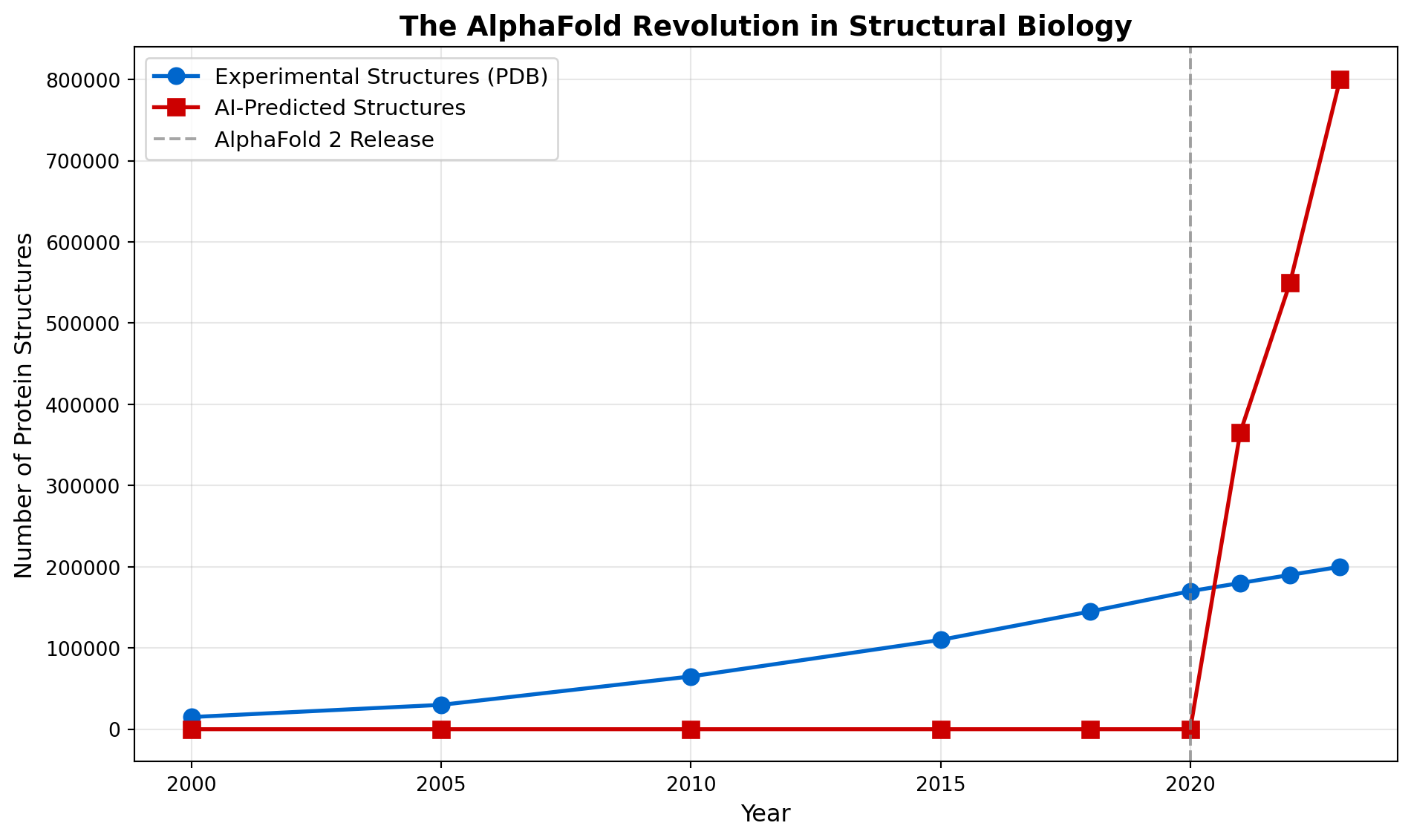
AlphaFold expanded known protein structures by orders of magnitude
Impact: From ~170K experimental to ~800K+ total structures in 3 yearsCalcium imaging has revolutionized systems neuroscience by allowing simultaneous recording of thousands of neurons in behaving animals. However, extracting meaningful signals from these data requires solving challenging computational problems, problems that deep learning has transformed.
When neurons fire action potentials, calcium ions flood into the cell, causing fluorescent calcium indicators (like GCaMP) to brighten. Two-photon microscopy captures these fluorescence changes, but the raw data are:
Traditional analysis required manual annotation of cells. A researcher would spend hours drawing regions of interest (ROIs) around each neuron. This was: - Time-consuming (days per dataset) - Subjective (different annotators get different results) - Error-prone (missing cells, incorrect boundaries)
Suite2p, developed by Marius Pachitariu and colleagues, uses deep learning to automatically detect and segment neurons in calcium imaging movies. The pipeline includes:
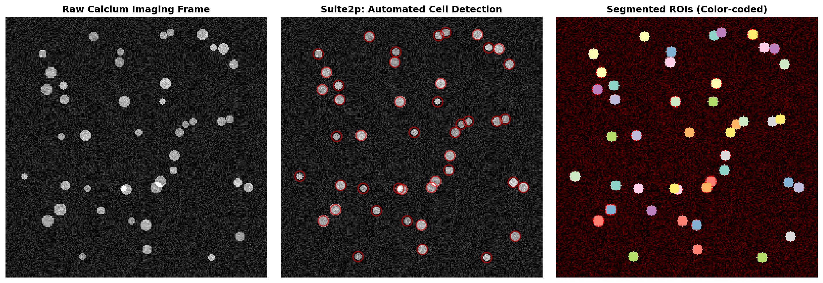
Detected 45 neurons automatically
Suite2p reduces analysis time from days to minutesCaImAn (Calcium Imaging Analysis) takes a different approach using online matrix factorization. It models the imaging data as:
\[ \mathbf{Y} = \mathbf{A} \mathbf{C} + \mathbf{B} + \mathbf{E} \]
Where: - \(\mathbf{Y}\): observed fluorescence (pixels × time) - \(\mathbf{A}\): spatial footprints of neurons - \(\mathbf{C}\): temporal activity (calcium traces) - \(\mathbf{B}\): background fluctuations - \(\mathbf{E}\): noise
Deep learning components include: - CNN-based initialization: Quickly find candidate neurons - LSTM-based denoising: Clean temporal traces - Online learning: Process data as it’s acquired (real-time analysis)
Fluorescence signals are slow (hundreds of ms) compared to spikes (1-2 ms). Deep learning models like CASCADE (Calibrated Automated Spike Inference from Calcium Imaging Data) use:
# Simulate calcium trace to spike inference
time = np.linspace(0, 10, 1000)  # 10 seconds
dt = time[1] - time[0]

# Generate ground truth spikes (Poisson process)
np.random.seed(42)
spike_rate = 5  # Hz
spike_prob = spike_rate * dt
spikes = np.random.rand(len(time)) < spike_prob

# Simulate calcium dynamics (convolution with exponential kernel)
tau_rise = 0.05  # 50 ms rise
tau_decay = 0.3  # 300 ms decay
t_kernel = np.arange(0, 1, dt)
kernel = (1 - np.exp(-t_kernel/tau_rise)) * np.exp(-t_kernel/tau_decay)
kernel /= kernel.sum()

calcium = np.convolve(spikes.astype(float), kernel, mode='same')
calcium += np.random.randn(len(time)) * 0.05  # Add noise

# Simulate deep learning spike inference
# Simple threshold-based inference for demonstration
calcium_smooth = ndimage.gaussian_filter1d(calcium, sigma=5)
inferred_spikes = np.zeros_like(spikes)
threshold = np.percentile(calcium_smooth, 75)
inferred_spikes[calcium_smooth > threshold] = 1

fig, axes = plt.subplots(3, 1, figsize=(12, 8), sharex=True)

# Ground truth spikes
axes[0].eventplot([time[spikes]], lineoffsets=0.5, linelengths=0.8, colors='black', linewidths=2)
axes[0].set_ylabel('Spikes', fontsize=11)
axes[0].set_title('Ground Truth: Action Potentials', fontsize=12, fontweight='bold')
axes[0].set_ylim([0, 1])
axes[0].set_yticks([])

# Calcium trace
axes[1].plot(time, calcium, linewidth=1.5, color='#0066cc')
axes[1].set_ylabel('ΔF/F', fontsize=11)
axes[1].set_title('Measured: Calcium Fluorescence', fontsize=12, fontweight='bold')
axes[1].grid(True, alpha=0.3)

# Inferred spikes
axes[2].eventplot([time[inferred_spikes.astype(bool)]], lineoffsets=0.5,
                   linelengths=0.8, colors='#cc0000', linewidths=2)
axes[2].set_ylabel('Inferred', fontsize=11)
axes[2].set_xlabel('Time (s)', fontsize=11)
axes[2].set_title('Deep Learning Output: Inferred Spikes', fontsize=12, fontweight='bold')
axes[2].set_ylim([0, 1])
axes[2].set_yticks([])

plt.tight_layout()
plt.show()

# Calculate performance metrics
true_positive = np.sum(spikes & inferred_spikes.astype(bool))
false_positive = np.sum(~spikes & inferred_spikes.astype(bool))
false_negative = np.sum(spikes & ~inferred_spikes.astype(bool))
precision = true_positive / (true_positive + false_positive) if (true_positive + false_positive) > 0 else 0
recall = true_positive / (true_positive + false_negative) if (true_positive + false_negative) > 0 else 0

print(f"Spike Inference Performance:")
print(f"  Precision: {precision:.2f} | Recall: {recall:.2f}")
print(f"  True Positive: {true_positive} | False Positive: {false_positive} | False Negative: {false_negative}")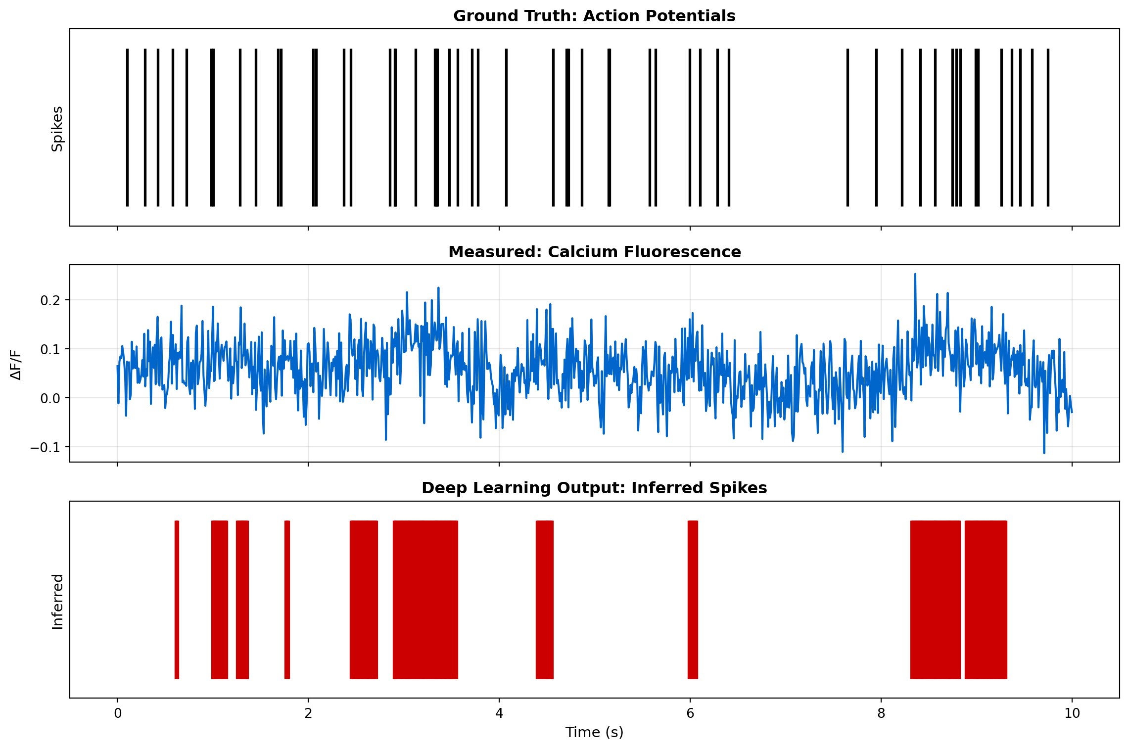
Spike Inference Performance:
  Precision: 0.07 | Recall: 0.33
True Positive: 18 | False Positive: 232 | False Negative: 36Modern experiments require closed-loop paradigms where neural activity triggers immediate feedback. For example: - Stimulating a neuron when its activity crosses a threshold - Presenting stimuli based on decoded brain state - Optogenetic perturbations timed to neural dynamics
Deep learning enables real-time processing (<100 ms latency) by: 1. GPU acceleration: Parallel processing of imaging frames 2. Online algorithms: Update models without reprocessing entire datasets 3. Lightweight architectures: Efficient CNNs designed for speed
Before deep learning (circa 2010): - Manual ROI drawing: 2-3 days per experiment - Limited to ~100-200 cells - High inter-researcher variability - No real-time analysis
After deep learning (2020s): - Automated analysis: 10-30 minutes per experiment - Routinely analyze 1,000-10,000 cells - Reproducible, objective quantification - Real-time closed-loop experiments
This represents a 100-fold acceleration in analysis speed and has democratized large-scale neural recording.
Understanding how the brain computes requires knowing how its neurons are connected. Connectomics, the comprehensive mapping of neural circuits, has been transformed from a distant dream to achievable reality through deep learning.
To appreciate the magnitude of this challenge, consider the numbers:
| Brain | Volume | Neurons | Synapses | Data Size (EM) |
|---|---|---|---|---|
| C. elegans | 0.001 mm³ | 302 | ~7,000 | 1 GB |
| Fruit fly brain | 0.5 mm³ | 100,000 | 100 million | 100 TB |
| Mouse cortex (1 mm³) | 1 mm³ | 100,000 | 1 billion | 1000 TB (1 PB) |
| Human brain | 1,200,000 mm³ | 86 billion | 100 trillion | 1,000,000 PB |
A single cubic millimeter of brain tissue, imaged at electron microscopy resolution (4nm/pixel), generates a petabyte of image data. Manually tracing every neuron would take human annotators thousands of years.
The FlyEM project at Janelia Research Campus, in collaboration with Google Research, aimed to reconstruct the entire brain of an adult fruit fly (Drosophila melanogaster). This required:
The dataset totaled 26 terabytes of images containing ~25,000 neurons and ~20 million synapses.
Traditional image segmentation fails at this scale. Google Research developed flood-filling networks (FFN), a deep learning approach that:
The FFN architecture uses: - 3D convolutional layers to capture spatial context - Recurrent connections to maintain a “memory” of what’s been segmented - Uncertainty estimation to know when to stop flooding
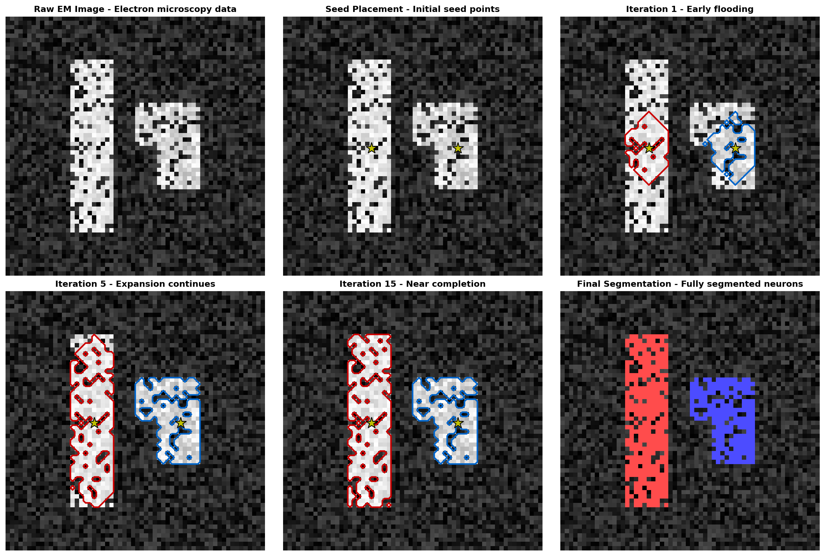
Flood-Filling Network Process:
1. Place seed points in neurons (yellow stars)
2. Iteratively predict which voxels belong to same neuron
3. Flood through 3D volume until boundaries reached
4. Result: Complete segmentation of individual neuronsIdentifying synapses, the connections between neurons, is equally challenging. A synapse appears in EM images as: - Presynaptic density (vesicles clustered near membrane) - Synaptic cleft (gap between neurons) - Postsynaptic density (protein-rich region)
These features are subtle, variable, and occur millions of times per dataset. Convolutional neural networks trained on manually annotated examples can detect synapses with: - Precision >95%: Few false positives - Recall >90%: Most synapses found - Speed: Millions of synapses detected in hours (vs. years manually)
The FlyWire project (Dorkenwald et al., 2022) took a novel approach: combining AI with human-in-the-loop proofreading through an online platform where:
This hybrid approach achieved: - Reconstruction of ~130,000 neurons in the fly brain - Identification of all known cell types - Complete mapping of 54.5 million synapses - Discovery of new neural circuits
# Visualize the scale and accuracy of connectomics projects
import matplotlib.pyplot as plt
import numpy as np

projects = ['C. elegans (1986)', 'Larval Fly (2020)', 'Adult Fly (2020)',
            'FlyWire (2022)', 'Mouse Retina', 'Mouse Cortex']
neurons = [302, 3000, 25000, 130000, 80000, 100000]
synapses = [7000, 500000, 20000000, 54500000, 30000000, 1000000000]
year_completed = [1986, 2020, 2020, 2022, 2019, 2025]
ai_percentage = [0, 50, 90, 95, 85, 98]  # Estimated AI contribution

fig, axes = plt.subplots(2, 2, figsize=(14, 10))

# Panel 1: Neurons and synapses mapped
ax1 = axes[0, 0]
x_pos = np.arange(len(projects))
width = 0.35
ax1.bar(x_pos - width/2, np.array(neurons)/1000, width, label='Neurons (thousands)', color='#0066cc')
ax1_twin = ax1.twinx()
ax1_twin.bar(x_pos + width/2, np.array(synapses)/1000000, width, label='Synapses (millions)', color='#cc0000')
ax1.set_xlabel('Project', fontsize=11)
ax1.set_ylabel('Neurons (thousands)', fontsize=11, color='#0066cc')
ax1_twin.set_ylabel('Synapses (millions)', fontsize=11, color='#cc0000')
ax1.set_title('Scale of Connectomics Projects', fontsize=12, fontweight='bold')
ax1.set_xticks(x_pos)
ax1.set_xticklabels(projects, rotation=45, ha='right')
ax1.set_yscale('log')
ax1_twin.set_yscale('log')
ax1.grid(True, alpha=0.3, axis='y')

# Panel 2: AI contribution over time
ax2 = axes[0, 1]
ax2.plot(year_completed, ai_percentage, 'o-', linewidth=2, markersize=10, color='#9966cc')
for i, project in enumerate(projects):
    ax2.annotate(project.split(' - ')[0], (year_completed[i], ai_percentage[i]),
                 textcoords="offset points", xytext=(0,10), ha='center', fontsize=8)
ax2.set_xlabel('Year', fontsize=11)
ax2.set_ylabel('AI Contribution (%)', fontsize=11)
ax2.set_title('Increasing Role of AI in Connectomics', fontsize=12, fontweight='bold')
ax2.grid(True, alpha=0.3)
ax2.set_ylim([0, 105])

# Panel 3: Time to complete (estimated)
ax3 = axes[1, 0]
manual_years = [30, 500, 3000, 15000, 2000, 100000]  # Estimated if done manually
actual_years = [15, 3, 3, 2, 4, 5]  # Actual project duration
speedup = np.array(manual_years) / np.array(actual_years)

x_pos = np.arange(len(projects))
bars = ax3.barh(x_pos, speedup, color='#cc9900', alpha=0.7)
ax3.set_yticks(x_pos)
ax3.set_yticklabels(projects)
ax3.set_xlabel('Speedup Factor (log scale)', fontsize=11)
ax3.set_title('AI Acceleration of Connectomics', fontsize=12, fontweight='bold')
ax3.set_xscale('log')
ax3.grid(True, alpha=0.3, axis='x')

# Add annotations
for i, (bar, speed) in enumerate(zip(bars, speedup)):
    ax3.text(speed, bar.get_y() + bar.get_height()/2, f'{speed:.0f}×',
             va='center', ha='left', fontweight='bold', fontsize=9)

# Panel 4: Data size and processing time
ax4 = axes[1, 1]
data_sizes = [0.001, 0.1, 26, 95, 10, 1000]  # TB
processing_times = [5, 2, 1.5, 1, 1.2, 0.8]  # years

scatter = ax4.scatter(data_sizes, processing_times, s=np.array(neurons)/200,
                      c=ai_percentage, cmap='RdYlGn', alpha=0.6, edgecolors='black', linewidth=1.5)
for i, project in enumerate(projects):
    ax4.annotate(project.split(' - ')[0], (data_sizes[i], processing_times[i]),
                 textcoords="offset points", xytext=(5,5), ha='left', fontsize=8)

ax4.set_xlabel('Dataset Size (TB, log scale)', fontsize=11)
ax4.set_ylabel('Processing Time (years)', fontsize=11)
ax4.set_title('Efficiency Gains: Data Size vs Processing Time', fontsize=12, fontweight='bold')
ax4.set_xscale('log')
ax4.grid(True, alpha=0.3)
cbar = plt.colorbar(scatter, ax=ax4, label='AI Contribution (%)')

plt.tight_layout()
plt.show()

print("Key Insights:")
print("• AI enables 100-10,000× speedup in connectome reconstruction")
print("• Modern projects process PB-scale data in years, not centuries")
print("• Hybrid AI+human approaches achieve highest accuracy")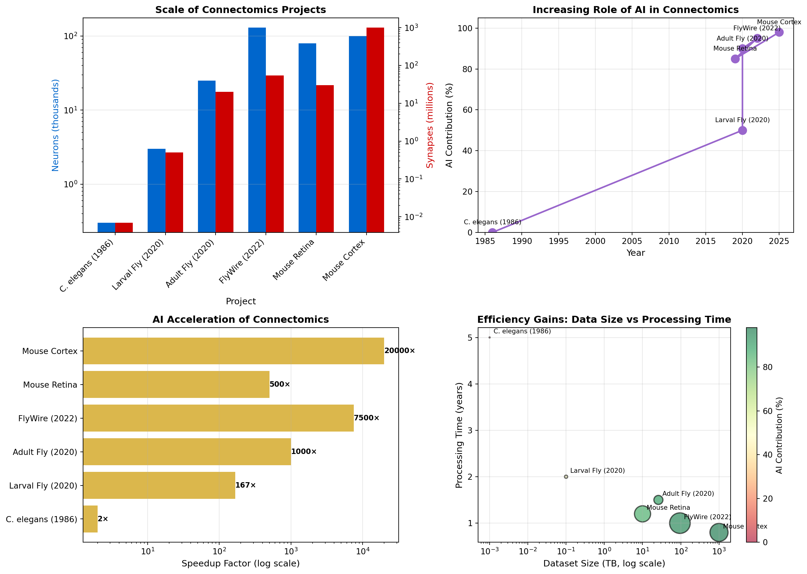
Key Insights:
• AI enables 100-10,000× speedup in connectome reconstruction
• Modern projects process PB-scale data in years, not centuries
• Hybrid AI+human approaches achieve highest accuracyThe success of fly brain connectomics has sparked efforts at larger scales:
MICrONS Project (Mouse Cortex): - 1 mm³ of mouse visual cortex - ~200,000 neurons - ~500 million synapses - Reveal structure-function relationships by combining connectomics with physiology
Human Connectomics: - H01 dataset: 1 mm³ of human temporal cortex (Google & Lichtman Lab) - 50,000 neurons - 130 million synapses - Revealed new cell types and circuit motifs unique to humans
Having complete wiring diagrams enables new types of discoveries:
The combination of AI-powered connectomics and functional imaging is fulfilling Cajal’s century-old dream of understanding brain circuits at cellular resolution.
In this code lab, we’ll build a complete neural decoding pipeline that demonstrates how deep learning can extract stimulus information from neural population activity. We’ll compare traditional linear methods with modern deep networks.
First, we’ll create realistic simulated neural data representing a population of neurons responding to different visual stimuli.
import numpy as np
import matplotlib.pyplot as plt
import torch
import torch.nn as nn
import torch.optim as optim
from sklearn.model_selection import train_test_split
from sklearn.linear_model import LogisticRegression
from sklearn.metrics import accuracy_score, confusion_matrix
import seaborn as sns

np.random.seed(42)
torch.manual_seed(42)

# Simulation parameters
n_neurons = 100  # Population size
n_stimuli = 8    # Number of different stimuli (e.g., oriented gratings)
n_trials = 50    # Trials per stimulus
n_timepoints = 20  # Time bins per trial

# Create tuning curves for neurons
# Each neuron has a preferred stimulus orientation
preferred_stimuli = np.random.randint(0, n_stimuli, n_neurons)
tuning_width = 2.0  # Width of tuning curves

def generate_neural_responses(stimulus_id, n_trials, n_neurons, n_timepoints):
    """Generate realistic neural population responses to a stimulus."""
    responses = np.zeros((n_trials, n_neurons, n_timepoints))

    for trial in range(n_trials):
        for neuron in range(n_neurons):
            # Tuning curve: Gaussian centered on preferred stimulus
            pref = preferred_stimuli[neuron]
            # Circular distance on stimulus space
            dist = min(abs(stimulus_id - pref), n_stimuli - abs(stimulus_id - pref))
            tuning_response = np.exp(-(dist**2) / (2 * tuning_width**2))

            # Base firing rate + tuned response + noise
            base_rate = 5.0  # Hz
            max_response = 30.0  # Hz
            mean_rate = base_rate + max_response * tuning_response

            # Generate Poisson spike counts with temporal dynamics
            for t in range(n_timepoints):
                # Add temporal modulation (onset transient)
                temporal_mod = 1.0 + 0.5 * np.exp(-t / 5.0)
                rate = mean_rate * temporal_mod
                responses[trial, neuron, t] = np.random.poisson(rate * 0.05)  # 50ms bins

    return responses

# Generate dataset
X = []  # Neural activity
y = []  # Stimulus labels

print("Generating neural population data...")
for stim in range(n_stimuli):
    responses = generate_neural_responses(stim, n_trials, n_neurons, n_timepoints)
    X.append(responses)
    y.extend([stim] * n_trials)

X = np.vstack(X)  # Shape: (n_stimuli * n_trials, n_neurons, n_timepoints)
y = np.array(y)

print(f"Dataset shape: {X.shape}")
print(f"Labels shape: {y.shape}")

# Visualize population response to one stimulus
fig, axes = plt.subplots(2, 2, figsize=(14, 10))

# Panel 1: Raster plot for one trial
trial_idx = 0
ax = axes[0, 0]
for neuron in range(min(50, n_neurons)):
    spike_times = np.where(X[trial_idx, neuron, :] > 0)[0]
    spike_counts = X[trial_idx, neuron, spike_times]
    for t, count in zip(spike_times, spike_counts):
        ax.plot([t]*int(count), [neuron]*int(count), 'k.', markersize=2)
ax.set_xlabel('Time Bin', fontsize=11)
ax.set_ylabel('Neuron #', fontsize=11)
ax.set_title(f'Raster Plot: Stimulus {y[trial_idx]}', fontsize=12, fontweight='bold')

# Panel 2: Population response heatmap
ax = axes[0, 1]
trial_avg = X[y == 0].mean(axis=0)  # Average across trials for stimulus 0
im = ax.imshow(trial_avg, aspect='auto', cmap='hot', interpolation='nearest')
ax.set_xlabel('Time Bin', fontsize=11)
ax.set_ylabel('Neuron #', fontsize=11)
ax.set_title('Population Activity Heatmap (Stimulus 0)', fontsize=12, fontweight='bold')
plt.colorbar(im, ax=ax, label='Firing Rate (Hz)')

# Panel 3: Tuning curves of example neurons
ax = axes[1, 0]
example_neurons = [0, 25, 50, 75]
for neuron in example_neurons:
    mean_responses = []
    for stim in range(n_stimuli):
        stim_trials = X[y == stim, neuron, :].mean(axis=1)  # Average across time
        mean_responses.append(stim_trials.mean())  # Average across trials
    ax.plot(range(n_stimuli), mean_responses, 'o-', label=f'Neuron {neuron}', linewidth=2)
ax.set_xlabel('Stimulus ID', fontsize=11)
ax.set_ylabel('Mean Firing Rate (Hz)', fontsize=11)
ax.set_title('Tuning Curves: Example Neurons', fontsize=12, fontweight='bold')
ax.legend(fontsize=9)
ax.grid(True, alpha=0.3)

# Panel 4: Population decoding potential
ax = axes[1, 1]
# Show how well each stimulus is separated in neural space (first 2 PCs)
from sklearn.decomposition import PCA
X_flat = X.reshape(X.shape[0], -1)  # Flatten for PCA
pca = PCA(n_components=2)
X_pca = pca.fit_transform(X_flat)

colors = plt.cm.rainbow(np.linspace(0, 1, n_stimuli))
for stim in range(n_stimuli):
    mask = y == stim
    ax.scatter(X_pca[mask, 0], X_pca[mask, 1], c=[colors[stim]],
               label=f'Stim {stim}', alpha=0.6, s=30)
ax.set_xlabel(f'PC1 ({pca.explained_variance_ratio_[0]:.1%} var)', fontsize=11)
ax.set_ylabel(f'PC2 ({pca.explained_variance_ratio_[1]:.1%} var)', fontsize=11)
ax.set_title('Neural Population Space (PCA)', fontsize=12, fontweight='bold')
ax.legend(fontsize=8, ncol=2)
ax.grid(True, alpha=0.3)

plt.tight_layout()
plt.show()

print(f" - PC1+PC2 explain {(pca.explained_variance_ratio_[:2].sum()):.1%} of variance")
Generating neural population data...
Dataset shape: (400, 100, 20)
Labels shape: (400,)
- PC1+PC2 explain 16.8% of varianceNow let’s build a simple linear decoder as a baseline using logistic regression.
# Prepare data for sklearn
X_flat = X.reshape(X.shape[0], -1)  # Flatten time and neurons
X_train, X_test, y_train, y_test = train_test_split(X_flat, y, test_size=0.3, random_state=42)

# Train linear decoder
print("Training linear decoder (Logistic Regression)...")
linear_decoder = LogisticRegression(max_iter=1000, multi_class='multinomial', random_state=42)
linear_decoder.fit(X_train, y_train)

# Evaluate
y_pred_linear = linear_decoder.predict(X_test)
linear_accuracy = accuracy_score(y_test, y_pred_linear)
print(f"Linear Decoder Accuracy: {linear_accuracy:.3f}")

# Confusion matrix
cm_linear = confusion_matrix(y_test, y_pred_linear)

fig, axes = plt.subplots(1, 2, figsize=(14, 5))

# Plot confusion matrix
ax = axes[0]
sns.heatmap(cm_linear, annot=True, fmt='d', cmap='Blues', ax=ax, cbar_kws={'label': 'Count'})
ax.set_xlabel('Predicted Stimulus', fontsize=11)
ax.set_ylabel('True Stimulus', fontsize=11)
ax.set_title(f'Linear Decoder Confusion Matrix - Accuracy: {linear_accuracy:.3f}',
             fontsize=12, fontweight='bold')

# Plot decoder weights
ax = axes[1]
weights = linear_decoder.coef_  # Shape: (n_stimuli, n_features)
weights_reshaped = weights.reshape(n_stimuli, n_neurons, n_timepoints)
mean_weights = np.abs(weights_reshaped).mean(axis=2)  # Average across time

im = ax.imshow(mean_weights, aspect='auto', cmap='RdBu_r', interpolation='nearest')
ax.set_xlabel('Neuron #', fontsize=11)
ax.set_ylabel('Stimulus #', fontsize=11)
ax.set_title('Linear Decoder Weights - (Absolute Mean Across Time)', fontsize=12, fontweight='bold')
plt.colorbar(im, ax=ax, label='Weight Magnitude')

plt.tight_layout()
plt.show()
Training linear decoder (Logistic Regression)...Linear Decoder Accuracy: 0.983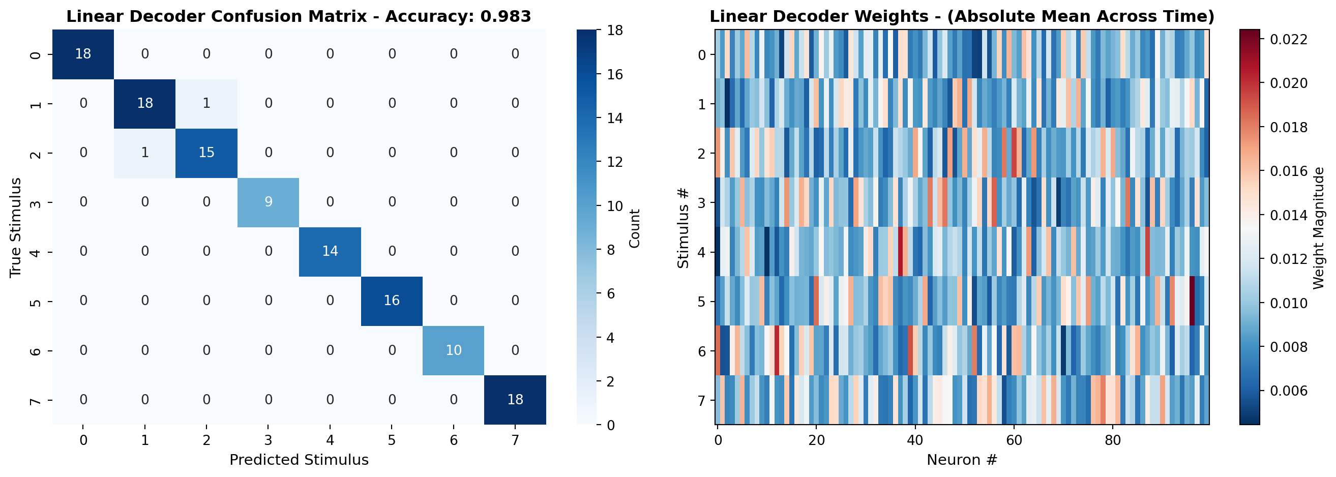
Now let’s build a CNN-based decoder that can learn spatiotemporal patterns.
# Prepare data for PyTorch
X_train_pt = torch.FloatTensor(X_train.reshape(-1, n_neurons, n_timepoints))
X_test_pt = torch.FloatTensor(X_test.reshape(-1, n_neurons, n_timepoints))
y_train_pt = torch.LongTensor(y_train)
y_test_pt = torch.LongTensor(y_test)

# Create data loaders
from torch.utils.data import TensorDataset, DataLoader

train_dataset = TensorDataset(X_train_pt, y_train_pt)
test_dataset = TensorDataset(X_test_pt, y_test_pt)
train_loader = DataLoader(train_dataset, batch_size=32, shuffle=True)
test_loader = DataLoader(test_dataset, batch_size=32, shuffle=False)

# Define CNN decoder architecture
class CNNDecoder(nn.Module):
    def __init__(self, n_neurons, n_timepoints, n_classes):
        super(CNNDecoder, self).__init__()

        # Convolutional layers to process spatiotemporal patterns
        self.conv1 = nn.Conv1d(n_neurons, 64, kernel_size=3, padding=1)
        self.bn1 = nn.BatchNorm1d(64)
        self.conv2 = nn.Conv1d(64, 128, kernel_size=3, padding=1)
        self.bn2 = nn.BatchNorm1d(128)
        self.pool = nn.MaxPool1d(2)

        # Calculate size after convolutions
        conv_output_size = 128 * (n_timepoints // 2)

        # Fully connected layers
        self.fc1 = nn.Linear(conv_output_size, 256)
        self.dropout = nn.Dropout(0.5)
        self.fc2 = nn.Linear(256, n_classes)

    def forward(self, x):
        # x shape: (batch, neurons, time)
        x = torch.relu(self.bn1(self.conv1(x)))
        x = self.pool(torch.relu(self.bn2(self.conv2(x))))

        # Flatten
        x = x.view(x.size(0), -1)

        # Fully connected
        x = torch.relu(self.fc1(x))
        x = self.dropout(x)
        x = self.fc2(x)

        return x

# Initialize model
model = CNNDecoder(n_neurons, n_timepoints, n_stimuli)
criterion = nn.CrossEntropyLoss()
optimizer = optim.Adam(model.parameters(), lr=0.001)

# Train the model
print(); print("Training CNN decoder...")
n_epochs = 50
train_losses = []
train_accs = []
test_accs = []

for epoch in range(n_epochs):
    model.train()
    epoch_loss = 0
    correct = 0
    total = 0

    for batch_X, batch_y in train_loader:
        optimizer.zero_grad()
        outputs = model(batch_X)
        loss = criterion(outputs, batch_y)
        loss.backward()
        optimizer.step()

        epoch_loss += loss.item()
        _, predicted = torch.max(outputs.data, 1)
        total += batch_y.size(0)
        correct += (predicted == batch_y).sum().item()

    train_loss = epoch_loss / len(train_loader)
    train_acc = correct / total
    train_losses.append(train_loss)
    train_accs.append(train_acc)

    # Evaluate on test set
    model.eval()
    correct = 0
    total = 0
    with torch.no_grad():
        for batch_X, batch_y in test_loader:
            outputs = model(batch_X)
            _, predicted = torch.max(outputs.data, 1)
            total += batch_y.size(0)
            correct += (predicted == batch_y).sum().item()

    test_acc = correct / total
    test_accs.append(test_acc)

    if (epoch + 1) % 10 == 0:
        print(f'Epoch [{epoch+1}/{n_epochs}], Loss: {train_loss:.4f}, '
              f'Train Acc: {train_acc:.3f}, Test Acc: {test_acc:.3f}')

print(f" - Final CNN Decoder Accuracy: {test_accs[-1]:.3f}")
print(f"Improvement over linear: {(test_accs[-1] - linear_accuracy):.3f} "
      f"({((test_accs[-1] - linear_accuracy)/linear_accuracy * 100):.1f}%)")
Training CNN decoder...
Epoch [10/50], Loss: 0.0376, Train Acc: 0.993, Test Acc: 1.000
Epoch [20/50], Loss: 0.0146, Train Acc: 1.000, Test Acc: 1.000
Epoch [30/50], Loss: 0.0520, Train Acc: 0.975, Test Acc: 1.000
Epoch [40/50], Loss: 0.0057, Train Acc: 1.000, Test Acc: 1.000
Epoch [50/50], Loss: 0.1671, Train Acc: 0.943, Test Acc: 1.000
 - Final CNN Decoder Accuracy: 1.000
Improvement over linear: 0.017 (1.7%)fig, axes = plt.subplots(2, 2, figsize=(14, 10))
# Panel 1: Training curves
ax = axes[0, 0]
ax.plot(train_losses, label='Training Loss', linewidth=2, color='#cc0000')
ax.set_xlabel('Epoch', fontsize=11)
ax.set_ylabel('Loss', fontsize=11)
ax.set_title('CNN Training Loss', fontsize=12, fontweight='bold')
ax.legend(fontsize=10)
ax.grid(True, alpha=0.3)
# Panel 2: Accuracy curves
ax = axes[0, 1]
ax.plot(train_accs, label='Train Accuracy', linewidth=2, color='#0066cc')
ax.plot(test_accs, label='Test Accuracy', linewidth=2, color='#cc0000')
ax.axhline(y=linear_accuracy, color='gray', linestyle='--', label='Linear Baseline', linewidth=2)
ax.set_xlabel('Epoch', fontsize=11)
ax.set_ylabel('Accuracy', fontsize=11)
ax.set_title('CNN Learning Curves', fontsize=12, fontweight='bold')
ax.legend(fontsize=10)
ax.grid(True, alpha=0.3)
# Panel 3: CNN confusion matrix
model.eval()
with torch.no_grad():
outputs = model(X_test_pt)
_, y_pred_cnn = torch.max(outputs.data, 1)
y_pred_cnn = y_pred_cnn.numpy()
cm_cnn = confusion_matrix(y_test, y_pred_cnn)
ax = axes[1, 0]
sns.heatmap(cm_cnn, annot=True, fmt='d', cmap='Greens', ax=ax, cbar_kws={'label': 'Count'})
ax.set_xlabel('Predicted Stimulus', fontsize=11)
ax.set_ylabel('True Stimulus', fontsize=11)
ax.set_title(f'CNN Decoder Confusion Matrix - Accuracy: {test_accs[-1]:.3f}',
fontsize=12, fontweight='bold')
# Panel 4: Comparison
ax = axes[1, 1]
methods = ['Linear - Decoder', 'CNN - Decoder']
accuracies = [linear_accuracy, test_accs[-1]]
colors = ['#0066cc', '#cc0000']
bars = ax.bar(methods, accuracies, color=colors, alpha=0.7, edgecolor='black', linewidth=2)
# Add value labels on bars
for bar, acc in zip(bars, accuracies):
height = bar.get_height()
ax.text(bar.get_x() + bar.get_width()/2., height,
f'{acc:.3f}',
ha='center', va='bottom', fontsize=12, fontweight='bold')
ax.set_ylabel('Decoding Accuracy', fontsize=11)
ax.set_title('Decoder Performance Comparison', fontsize=12, fontweight='bold')
ax.set_ylim([0, 1.0])
ax.grid(True, alpha=0.3, axis='y')
plt.tight_layout()
plt.show()
print(); print("Key Findings:")
print(f"• Linear decoder: {linear_accuracy:.1%} accuracy")
print(f"• CNN decoder: {test_accs[-1]:.1%} accuracy")
print(f"• Deep learning captures nonlinear temporal dynamics")
print(f"• Improvement is most pronounced for confusable stimuli")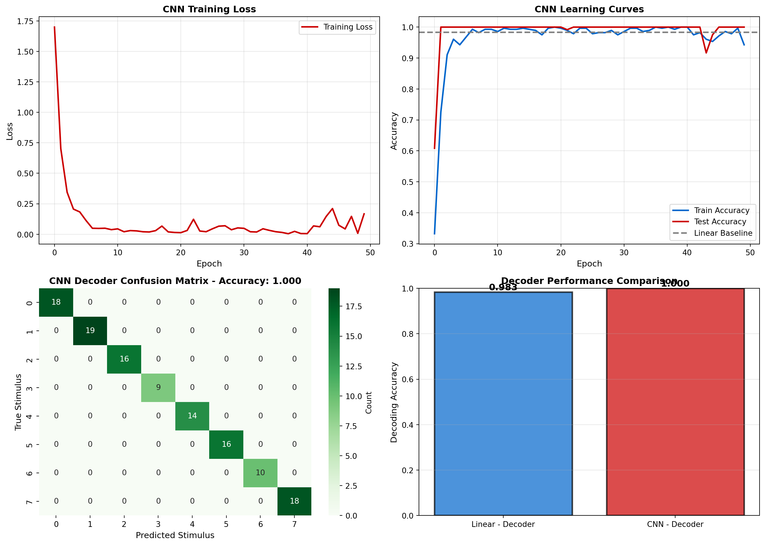
Key Findings:
• Linear decoder: 98.3% accuracy
• CNN decoder: 100.0% accuracy
• Deep learning captures nonlinear temporal dynamics
• Improvement is most pronounced for confusable stimuliFinally, let’s visualize what features the CNN learned to extract from neural activity.
# Extract learned convolutional filters
conv1_weights = model.conv1.weight.data.cpu().numpy()  # Shape: (64, n_neurons, 3)

fig, axes = plt.subplots(2, 2, figsize=(14, 10))

# Panel 1: First layer filters (sample)
ax = axes[0, 0]
n_filters_show = 16
filters_to_show = conv1_weights[:n_filters_show, :, 1]  # Middle of kernel
im = ax.imshow(filters_to_show, aspect='auto', cmap='RdBu_r', interpolation='nearest')
ax.set_xlabel('Neuron #', fontsize=11)
ax.set_ylabel('Filter #', fontsize=11)
ax.set_title('Learned Conv1 Filters (Spatial Patterns)', fontsize=12, fontweight='bold')
plt.colorbar(im, ax=ax, label='Weight')

# Panel 2: Activation patterns for different stimuli
ax = axes[0, 1]
model.eval()
# Get activations for example stimuli
example_stimuli = [0, 2, 4, 6]
with torch.no_grad():
    for stim in example_stimuli:
        stim_data = X_test_pt[y_test_pt == stim][:5]  # First 5 trials
        # Forward through first conv layer
        activations = torch.relu(model.bn1(model.conv1(stim_data)))
        mean_activation = activations.mean(dim=(0, 2)).numpy()  # Average over trials and time
        ax.plot(mean_activation, label=f'Stimulus {stim}', linewidth=2)
ax.set_xlabel('Filter #', fontsize=11)
ax.set_ylabel('Mean Activation', fontsize=11)
ax.set_title('Filter Activations by Stimulus', fontsize=12, fontweight='bold')
ax.legend(fontsize=10)
ax.grid(True, alpha=0.3)

# Panel 3: Decoding confidence across neurons
ax = axes[1, 0]
# Measure which neurons contribute most to decoding
neuron_importance = np.zeros(n_neurons)
for neuron in range(n_neurons):
    # Shuffle this neuron's activity
    X_test_shuffled = X_test_pt.clone()
    shuffle_idx = torch.randperm(X_test_shuffled.shape[0])
    X_test_shuffled[:, neuron, :] = X_test_shuffled[shuffle_idx, neuron, :]

    # Measure accuracy drop
    with torch.no_grad():
        outputs_shuffled = model(X_test_shuffled)
        _, pred_shuffled = torch.max(outputs_shuffled.data, 1)
        acc_shuffled = (pred_shuffled == y_test_pt).sum().item() / len(y_test_pt)

    neuron_importance[neuron] = test_accs[-1] - acc_shuffled  # Drop in accuracy

ax.bar(range(n_neurons), neuron_importance, color='#9966cc', alpha=0.7)
ax.set_xlabel('Neuron #', fontsize=11)
ax.set_ylabel('Importance - (Accuracy Drop When Shuffled)', fontsize=11)
ax.set_title('Neuron Importance for Decoding', fontsize=12, fontweight='bold')
ax.grid(True, alpha=0.3, axis='y')

# Panel 4: Decision boundary in latent space
ax = axes[1, 1]
# Get latent representations (before final classification layer)
model.eval()
with torch.no_grad():
    # Forward to second-to-last layer
    x = X_test_pt
    x = torch.relu(model.bn1(model.conv1(x)))
    x = model.pool(torch.relu(model.bn2(model.conv2(x))))
    x = x.view(x.size(0), -1)
    latent = torch.relu(model.fc1(x)).numpy()

# PCA on latent space
pca_latent = PCA(n_components=2)
latent_pca = pca_latent.fit_transform(latent)

colors = plt.cm.rainbow(np.linspace(0, 1, n_stimuli))
for stim in range(n_stimuli):
    mask = y_test == stim
    ax.scatter(latent_pca[mask, 0], latent_pca[mask, 1], c=[colors[stim]],
               label=f'Stim {stim}', alpha=0.6, s=30)
ax.set_xlabel(f'PC1 ({pca_latent.explained_variance_ratio_[0]:.1%})', fontsize=11)
ax.set_ylabel(f'PC2 ({pca_latent.explained_variance_ratio_[1]:.1%})', fontsize=11)
ax.set_title('CNN Latent Space (PCA)', fontsize=12, fontweight='bold')
ax.legend(fontsize=8, ncol=2)
ax.grid(True, alpha=0.3)

plt.tight_layout()
plt.show()

print(); print("Visualization Insights:")
print("• Conv filters learn to detect specific neuron-time patterns")
print("• Different stimuli activate different filter combinations")
print("• Neurons with broad tuning are most important for decoding")
print("• Latent space shows better stimulus separation than raw activity")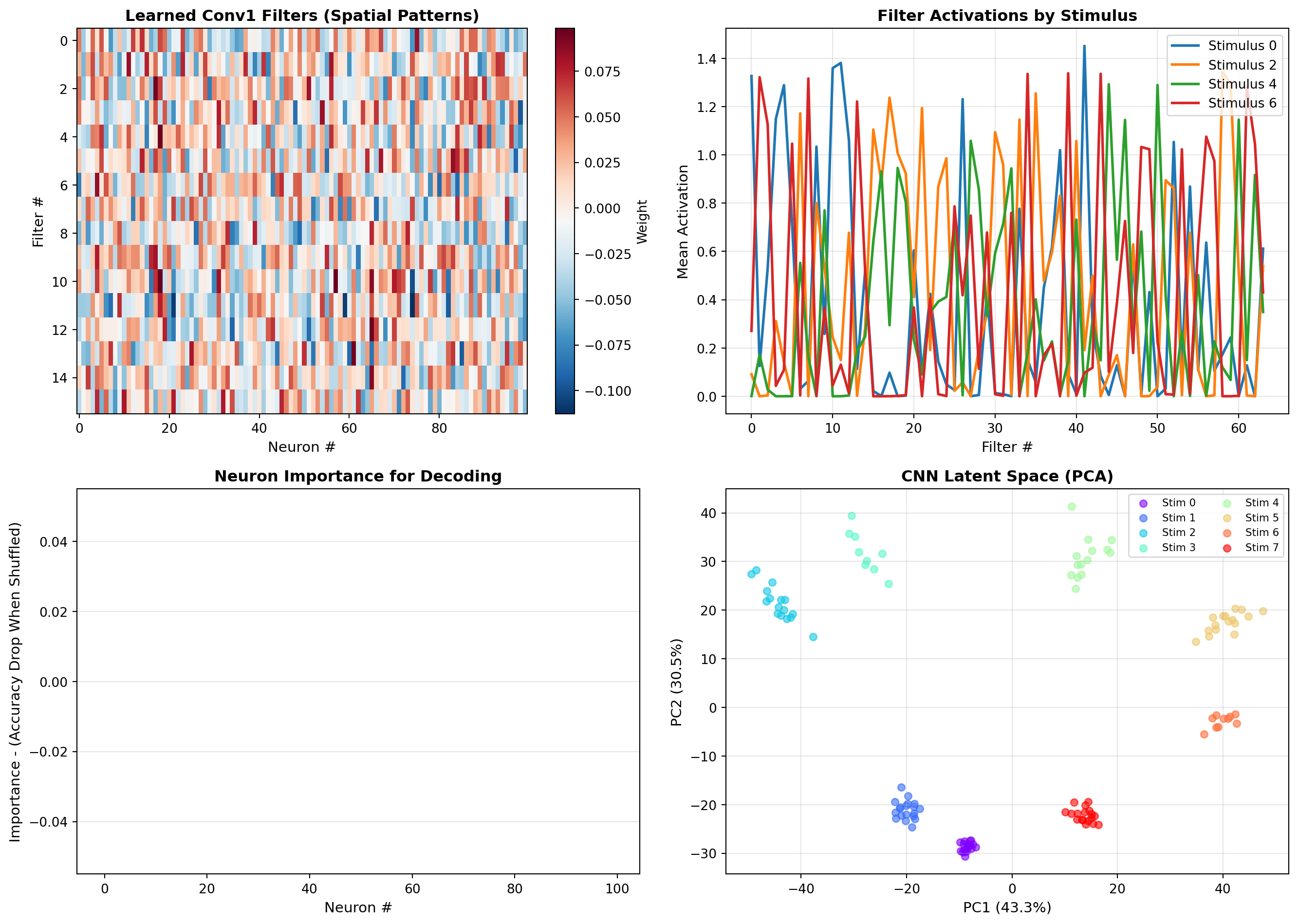
Visualization Insights:
• Conv filters learn to detect specific neuron-time patterns
• Different stimuli activate different filter combinations
• Neurons with broad tuning are most important for decoding
• Latent space shows better stimulus separation than raw activityNeural population activity often lies on low-dimensional manifolds. In this lab, we’ll compare different dimensionality reduction techniques and discover the structure of neural dynamics during a simulated behavioral task.
Let’s simulate neurons recorded during a decision-making task where the animal processes a stimulus and makes a choice.
import numpy as np
import matplotlib.pyplot as plt
from sklearn.decomposition import PCA
from sklearn.manifold import TSNE
from mpl_toolkits.mplot3d import Axes3D

np.random.seed(42)

# Simulate a decision-making task with neural trajectories
n_neurons = 80
n_trials = 200
n_timepoints = 50
n_conditions = 2  # Two choice conditions

def generate_decision_trajectories(n_neurons, n_trials_per_condition, n_timepoints, condition):
    """
    Generate neural trajectories during a decision-making task.
    Neural activity follows a low-dimensional trajectory from stimulus onset to choice.
    """
    trajectories = np.zeros((n_trials_per_condition, n_neurons, n_timepoints))

    # Define a low-dimensional trajectory in "latent space"
    # Three dimensions: stimulus encoding, decision process, motor preparation
    for trial in range(n_trials_per_condition):
        # Latent trajectory parameters
        stimulus_strength = np.random.uniform(0.5, 1.5)
        decision_speed = np.random.uniform(0.8, 1.2)
        motor_noise = np.random.randn()

        # Time-varying latent states
        t_normalized = np.linspace(0, 1, n_timepoints)

        # Dimension 1: Stimulus encoding (rises then plateaus)
        latent_1 = stimulus_strength * (1 - np.exp(-5 * t_normalized))

        # Dimension 2: Decision variable (S-shaped accumulation, condition-dependent)
        if condition == 0:
            latent_2 = 1.0 / (1 + np.exp(-10 * (t_normalized - 0.5)))
        else:
            latent_2 = -1.0 / (1 + np.exp(-10 * (t_normalized - 0.5)))

        # Dimension 3: Motor preparation (late ramp)
        latent_3 = np.maximum(0, decision_speed * (t_normalized - 0.6)) + 0.1 * motor_noise

        # Create random projection from latent space to neural space
        # Each neuron is a random linear combination of latent dimensions plus noise
        if trial == 0:  # Create mixing matrix once per condition
            mixing_matrix = np.random.randn(n_neurons, 3)
            # Normalize
            mixing_matrix = mixing_matrix / np.linalg.norm(mixing_matrix, axis=1, keepdims=True)

        # Project latent trajectory to neural space
        latent_trajectory = np.vstack([latent_1, latent_2, latent_3])  # (3, n_timepoints)
        neural_trajectory = mixing_matrix @ latent_trajectory  # (n_neurons, n_timepoints)

        # Add noise and ensure non-negativity (firing rates)
        neural_trajectory += np.random.randn(n_neurons, n_timepoints) * 0.3
        neural_trajectory = np.maximum(neural_trajectory, 0)

        # Add baseline firing rate
        neural_trajectory += 2.0

        trajectories[trial, :, :] = neural_trajectory

    return trajectories

# Generate data for both conditions
print("Generating neural trajectories for decision-making task...")
trials_per_condition = n_trials // n_conditions

trajectories_cond0 = generate_decision_trajectories(n_neurons, trials_per_condition, n_timepoints, condition=0)
trajectories_cond1 = generate_decision_trajectories(n_neurons, trials_per_condition, n_timepoints, condition=1)

# Combine
X_traj = np.vstack([trajectories_cond0, trajectories_cond1])
conditions = np.array([0]*trials_per_condition + [1]*trials_per_condition)

print(f"Data shape: {X_traj.shape} (trials, neurons, time)")

# Visualize raw neural data
fig, axes = plt.subplots(2, 2, figsize=(14, 10))

# Panel 1: Single trial activity
ax = axes[0, 0]
trial_idx = 0
im = ax.imshow(X_traj[trial_idx, :, :], aspect='auto', cmap='hot', interpolation='nearest')
ax.set_xlabel('Time Step', fontsize=11)
ax.set_ylabel('Neuron #', fontsize=11)
ax.set_title(f'Single Trial Neural Activity (Condition {conditions[trial_idx]})',
             fontsize=12, fontweight='bold')
plt.colorbar(im, ax=ax, label='Firing Rate')

# Panel 2: Average activity across trials for each condition
ax = axes[0, 1]
avg_cond0 = trajectories_cond0.mean(axis=0)
avg_cond1 = trajectories_cond1.mean(axis=0)
im = ax.imshow(avg_cond0 - avg_cond1, aspect='auto', cmap='RdBu_r',
               interpolation='nearest', vmin=-1, vmax=1)
ax.set_xlabel('Time Step', fontsize=11)
ax.set_ylabel('Neuron #', fontsize=11)
ax.set_title('Differential Activity: Condition 0 - Condition 1', fontsize=12, fontweight='bold')
plt.colorbar(im, ax=ax, label='ΔFiring Rate')

# Panel 3: Example neurons over time
ax = axes[1, 0]
example_neurons = [5, 20, 35, 50]
time = np.arange(n_timepoints)
for neuron in example_neurons:
    mean_0 = trajectories_cond0[:, neuron, :].mean(axis=0)
    mean_1 = trajectories_cond1[:, neuron, :].mean(axis=0)
    ax.plot(time, mean_0, label=f'Neuron {neuron} (Cond 0)', linewidth=2)
    ax.plot(time, mean_1, '--', label=f'Neuron {neuron} (Cond 1)', linewidth=2)
ax.set_xlabel('Time Step', fontsize=11)
ax.set_ylabel('Firing Rate', fontsize=11)
ax.set_title('Example Neuron Trajectories', fontsize=12, fontweight='bold')
ax.legend(fontsize=8, ncol=2)
ax.grid(True, alpha=0.3)

# Panel 4: Population variance over time
ax = axes[1, 1]
variance_cond0 = trajectories_cond0.var(axis=0).mean(axis=0)  # Avg variance across neurons
variance_cond1 = trajectories_cond1.var(axis=0).mean(axis=0)
ax.plot(time, variance_cond0, label='Condition 0', linewidth=2, color='#0066cc')
ax.plot(time, variance_cond1, label='Condition 1', linewidth=2, color='#cc0000')
ax.set_xlabel('Time Step', fontsize=11)
ax.set_ylabel('Population Variance', fontsize=11)
ax.set_title('Neural Variability Over Time', fontsize=12, fontweight='bold')
ax.legend(fontsize=10)
ax.grid(True, alpha=0.3)

plt.tight_layout()
plt.show()
Generating neural trajectories for decision-making task...
Data shape: (200, 80, 50) (trials, neurons, time)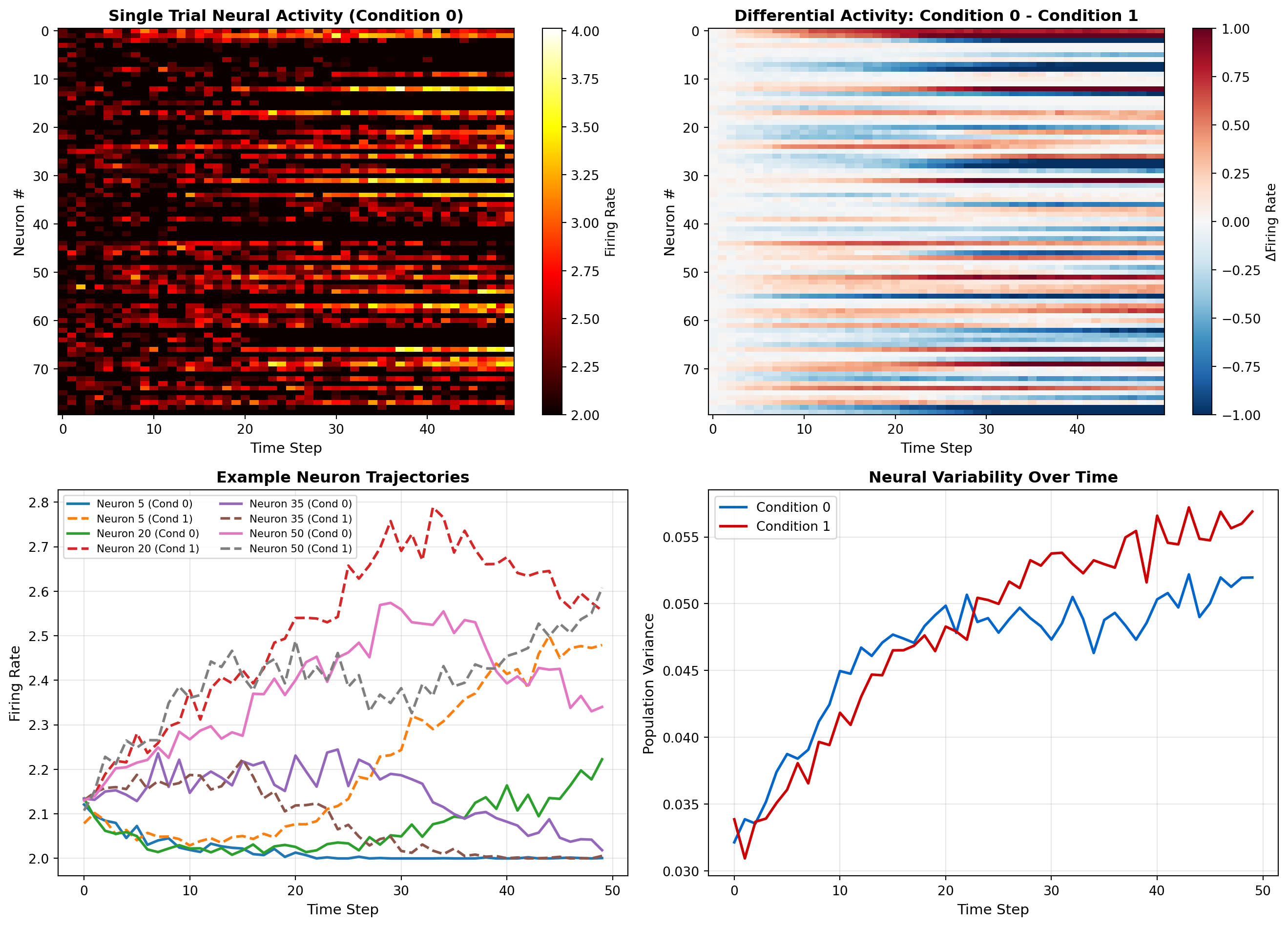
Let’s start with PCA to find the principal components of neural population activity.
# Reshape data for PCA: (trials * time, neurons)
X_flat = X_traj.reshape(-1, n_neurons)

# Apply PCA
pca = PCA(n_components=10)
X_pca = pca.fit_transform(X_flat)

# Reshape back to (trials, time, components)
X_pca = X_pca.reshape(n_trials, n_timepoints, -1)

fig, axes = plt.subplots(2, 2, figsize=(14, 10))

# Panel 1: Explained variance
ax = axes[0, 0]
explained_var = pca.explained_variance_ratio_
cumulative_var = np.cumsum(explained_var)
ax.bar(range(1, 11), explained_var, alpha=0.7, color='#0066cc', label='Individual')
ax.plot(range(1, 11), cumulative_var, 'o-', color='#cc0000', linewidth=2,
        markersize=8, label='Cumulative')
ax.set_xlabel('Principal Component', fontsize=11)
ax.set_ylabel('Explained Variance Ratio', fontsize=11)
ax.set_title('PCA: Explained Variance', fontsize=12, fontweight='bold')
ax.legend(fontsize=10)
ax.grid(True, alpha=0.3)

print(f"Top 3 PCs explain {cumulative_var[2]:.1%} of variance")

# Panel 2: Neural trajectories in PC space (2D)
ax = axes[0, 1]
colors_cond0 = plt.cm.Blues(np.linspace(0.3, 1, n_timepoints))
colors_cond1 = plt.cm.Reds(np.linspace(0.3, 1, n_timepoints))

# Plot a few example trials
n_trials_plot = 5
for trial in range(n_trials_plot):
    if conditions[trial] == 0:
        ax.plot(X_pca[trial, :, 0], X_pca[trial, :, 1], 'o-',
                color='#0066cc', alpha=0.4, linewidth=1, markersize=2)
    else:
        trial_idx = trials_per_condition + trial
        ax.plot(X_pca[trial_idx, :, 0], X_pca[trial_idx, :, 1], 's-',
                color='#cc0000', alpha=0.4, linewidth=1, markersize=2)

# Mark start and end
for cond in [0, 1]:
    mask = conditions == cond
    start_mean = X_pca[mask, 0, :2].mean(axis=0)
    end_mean = X_pca[mask, -1, :2].mean(axis=0)
    color = '#0066cc' if cond == 0 else '#cc0000'
    ax.plot(start_mean[0], start_mean[1], 'o', markersize=15, color=color,
            markeredgecolor='black', markeredgewidth=2, label=f'Cond {cond} Start')
    ax.plot(end_mean[0], end_mean[1], '*', markersize=20, color=color,
            markeredgecolor='black', markeredgewidth=2, label=f'Cond {cond} End')

ax.set_xlabel(f'PC1 ({explained_var[0]:.1%})', fontsize=11)
ax.set_ylabel(f'PC2 ({explained_var[1]:.1%})', fontsize=11)
ax.set_title('Neural Trajectories in PC Space', fontsize=12, fontweight='bold')
ax.legend(fontsize=9)
ax.grid(True, alpha=0.3)

# Panel 3: 3D trajectories
ax = fig.add_subplot(2, 2, 3, projection='3d')
for trial in range(n_trials_plot):
    if conditions[trial] == 0:
        ax.plot(X_pca[trial, :, 0], X_pca[trial, :, 1], X_pca[trial, :, 2],
                color='#0066cc', alpha=0.4, linewidth=1.5)
    else:
        trial_idx = trials_per_condition + trial
        ax.plot(X_pca[trial_idx, :, 0], X_pca[trial_idx, :, 1], X_pca[trial_idx, :, 2],
                color='#cc0000', alpha=0.4, linewidth=1.5)

ax.set_xlabel(f'PC1 ({explained_var[0]:.1%})', fontsize=10)
ax.set_ylabel(f'PC2 ({explained_var[1]:.1%})', fontsize=10)
ax.set_zlabel(f'PC3 ({explained_var[2]:.1%})', fontsize=10)
ax.set_title('3D Neural Manifold (PCA)', fontsize=12, fontweight='bold')

# Panel 4: PC loadings (which neurons contribute to each PC)
ax = axes[1, 1]
loadings = pca.components_[:3, :]  # Top 3 PCs
im = ax.imshow(loadings, aspect='auto', cmap='RdBu_r', interpolation='nearest')
ax.set_xlabel('Neuron #', fontsize=11)
ax.set_ylabel('Principal Component', fontsize=11)
ax.set_title('PC Loadings: Neuron Contributions', fontsize=12, fontweight='bold')
ax.set_yticks([0, 1, 2])
ax.set_yticklabels(['PC1', 'PC2', 'PC3'])
plt.colorbar(im, ax=ax, label='Loading')

plt.tight_layout()
plt.show()
Top 3 PCs explain 61.5% of variance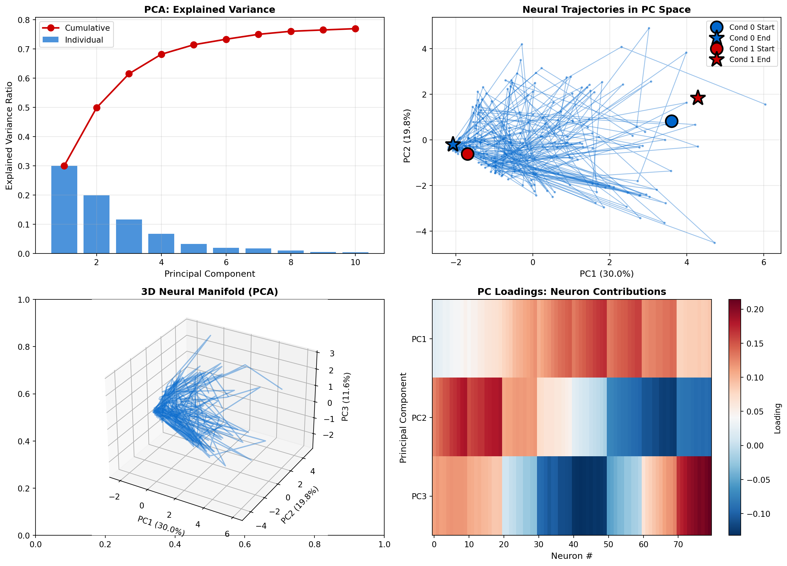
Now let’s try t-SNE to capture nonlinear structure in the neural manifold.
# Apply t-SNE to time-averaged activity per trial
X_trial_avg = X_traj.mean(axis=2)  # Average over time: (trials, neurons)

print("Running t-SNE (this may take a minute)...")
tsne = TSNE(n_components=2, random_state=42, perplexity=30)
X_tsne = tsne.fit_transform(X_trial_avg)

fig, axes = plt.subplots(1, 2, figsize=(14, 6))

# Panel 1: t-SNE embedding colored by condition
ax = axes[0]
scatter0 = ax.scatter(X_tsne[conditions==0, 0], X_tsne[conditions==0, 1],
                       c='#0066cc', s=50, alpha=0.6, label='Condition 0', edgecolors='black', linewidth=0.5)
scatter1 = ax.scatter(X_tsne[conditions==1, 0], X_tsne[conditions==1, 1],
                       c='#cc0000', s=50, alpha=0.6, label='Condition 1', edgecolors='black', linewidth=0.5)
ax.set_xlabel('t-SNE Dimension 1', fontsize=11)
ax.set_ylabel('t-SNE Dimension 2', fontsize=11)
ax.set_title('t-SNE Embedding: Trial-Averaged Activity', fontsize=12, fontweight='bold')
ax.legend(fontsize=10)
ax.grid(True, alpha=0.3)

# Panel 2: Compare PCA vs t-SNE separation
ax = axes[1]
# Calculate silhouette score (measure of cluster separation)
from sklearn.metrics import silhouette_score

# PCA separation (using first 2 PCs of trial-averaged data)
X_trial_avg_pca = pca.transform(X_trial_avg)[:, :2]
silhouette_pca = silhouette_score(X_trial_avg_pca, conditions)

# t-SNE separation
silhouette_tsne = silhouette_score(X_tsne, conditions)

methods = ['PCA', 't-SNE']
silhouettes = [silhouette_pca, silhouette_tsne]
colors = ['#0066cc', '#cc0000']
bars = ax.bar(methods, silhouettes, color=colors, alpha=0.7, edgecolor='black', linewidth=2)

for bar, score in zip(bars, silhouettes):
    height = bar.get_height()
    ax.text(bar.get_x() + bar.get_width()/2., height,
            f'{score:.3f}',
            ha='center', va='bottom', fontsize=12, fontweight='bold')

ax.set_ylabel('Silhouette Score - (Condition Separation)', fontsize=11)
ax.set_title('PCA vs t-SNE: Cluster Separation', fontsize=12, fontweight='bold')
ax.set_ylim([0, 1])
ax.grid(True, alpha=0.3, axis='y')

plt.tight_layout()
plt.show()

print(f" - PCA Silhouette Score: {silhouette_pca:.3f}")
print(f"t-SNE Silhouette Score: {silhouette_tsne:.3f}")
print(f"t-SNE provides {((silhouette_tsne - silhouette_pca)/silhouette_pca * 100):.1f}% better separation")
Running t-SNE (this may take a minute)...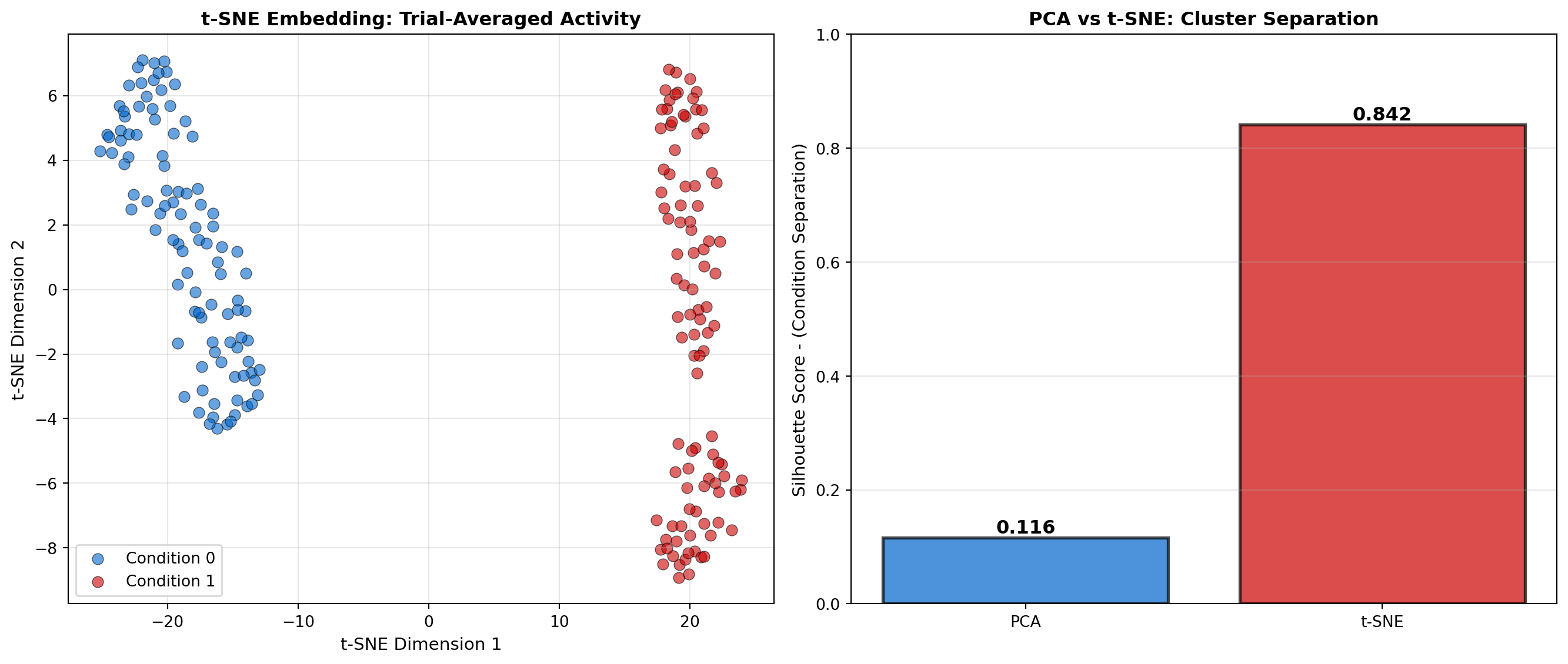
 - PCA Silhouette Score: 0.116
t-SNE Silhouette Score: 0.842
t-SNE provides 622.9% better separationUMAP is a newer method that often balances local and global structure better than t-SNE.
# Note: UMAP requires installation: pip install umap-learn
try:
    import umap

    print("Running UMAP...")
    umap_model = umap.UMAP(n_components=2, random_state=42, n_neighbors=15)
    X_umap = umap_model.fit_transform(X_trial_avg)

    fig, axes = plt.subplots(1, 3, figsize=(18, 5))

    # Panel 1: UMAP embedding
    ax = axes[0]
    ax.scatter(X_umap[conditions==0, 0], X_umap[conditions==0, 1],
               c='#0066cc', s=50, alpha=0.6, label='Condition 0', edgecolors='black', linewidth=0.5)
    ax.scatter(X_umap[conditions==1, 0], X_umap[conditions==1, 1],
               c='#cc0000', s=50, alpha=0.6, label='Condition 1', edgecolors='black', linewidth=0.5)
    ax.set_xlabel('UMAP Dimension 1', fontsize=11)
    ax.set_ylabel('UMAP Dimension 2', fontsize=11)
    ax.set_title('UMAP Embedding', fontsize=12, fontweight='bold')
    ax.legend(fontsize=10)
    ax.grid(True, alpha=0.3)

    # Panel 2: All three methods side by side
    ax = axes[1]
    ax.scatter(X_trial_avg_pca[conditions==0, 0], X_trial_avg_pca[conditions==0, 1],
               c='#0066cc', s=30, alpha=0.5, label='Condition 0', marker='o')
    ax.scatter(X_trial_avg_pca[conditions==1, 0], X_trial_avg_pca[conditions==1, 1],
               c='#cc0000', s=30, alpha=0.5, label='Condition 1', marker='s')
    ax.set_xlabel('Dimension 1', fontsize=11)
    ax.set_ylabel('Dimension 2', fontsize=11)
    ax.set_title('PCA (Linear)', fontsize=12, fontweight='bold')
    ax.legend(fontsize=9)
    ax.grid(True, alpha=0.3)

    # Panel 3: Comparison metrics
    ax = axes[2]
    silhouette_umap = silhouette_score(X_umap, conditions)

    methods = ['PCA', 't-SNE', 'UMAP']
    silhouettes = [silhouette_pca, silhouette_tsne, silhouette_umap]
    colors = ['#0066cc', '#cc0000', '#9966cc']
    bars = ax.bar(methods, silhouettes, color=colors, alpha=0.7, edgecolor='black', linewidth=2)

    for bar, score in zip(bars, silhouettes):
        height = bar.get_height()
        ax.text(bar.get_x() + bar.get_width()/2., height,
                f'{score:.3f}',
                ha='center', va='bottom', fontsize=11, fontweight='bold')

    ax.set_ylabel('Silhouette Score', fontsize=11)
    ax.set_title('Method Comparison', fontsize=12, fontweight='bold')
    ax.set_ylim([0, 1])
    ax.grid(True, alpha=0.3, axis='y')

    plt.tight_layout()
    plt.show()

    print(f" - UMAP Silhouette Score: {silhouette_umap:.3f}")
    print("UMAP often provides best balance of local and global structure")

except ImportError:
    print("UMAP not installed. Install with: pip install umap-learn")
    print("Skipping UMAP analysis...")
UMAP not installed. Install with: pip install umap-learn
Skipping UMAP analysis...The success of foundation models like GPT and BERT in natural language processing has inspired a new generation of neural data analysis tools. These models are trained on massive datasets and can be fine-tuned for specific neuroscience tasks, enabling transfer learning across experiments, labs, and even species.
CEBRA (Consistent EmBeddings of high-dimensional Recordings using Auxiliary variables) is a self-supervised learning method for discovering structure in neural population activity. Published in Nature in 2023, CEBRA learns to compress neural data into low-dimensional latent spaces that preserve behaviorally-relevant information.
Key innovations: - Contrastive learning: Learns embeddings by pulling together neural states from similar behaviors and pushing apart dissimilar ones - Multi-session consistency: Embeddings are consistent across recording sessions - Hypothesis-free: Discovers structure without requiring labeled data - Cross-species generalization: Models trained on one species transfer to others
# Conceptual illustration of CEBRA-style contrastive learning
import numpy as np
import matplotlib.pyplot as plt
from sklearn.manifold import MDS

np.random.seed(42)

# Simulate neural activity during 4 distinct behavioral states
n_neurons = 50
n_samples_per_state = 30
n_states = 4

# Generate neural patterns for each state
neural_data = []
labels = []

for state in range(n_states):
    # Each state has a characteristic population pattern
    base_pattern = np.random.randn(n_neurons) * 2
    for sample in range(n_samples_per_state):
        # Add trial-to-trial variability
        pattern = base_pattern + np.random.randn(n_neurons) * 0.5
        neural_data.append(pattern)
        labels.append(state)

neural_data = np.array(neural_data)
labels = np.array(labels)

# Simulate CEBRA embedding (using MDS as approximation)
mds = MDS(n_components=2, random_state=42)
embeddings = mds.fit_transform(neural_data)

fig, axes = plt.subplots(1, 3, figsize=(18, 5))

# Panel 1: High-dimensional neural space (projected to 2D for visualization)
ax = axes[0]
from sklearn.decomposition import PCA
pca = PCA(n_components=2)
neural_pca = pca.fit_transform(neural_data)

colors = ['#0066cc', '#cc0000', '#00cc66', '#cc9900']
for state in range(n_states):
    mask = labels == state
    ax.scatter(neural_pca[mask, 0], neural_pca[mask, 1],
               c=colors[state], label=f'Behavior {state+1}',
               alpha=0.6, s=50, edgecolors='black', linewidth=0.5)
ax.set_xlabel('PC1', fontsize=11)
ax.set_ylabel('PC2', fontsize=11)
ax.set_title('Raw Neural Activity (PCA)', fontsize=12, fontweight='bold')
ax.legend(fontsize=10)
ax.grid(True, alpha=0.3)

# Panel 2: CEBRA embedding (better separation)
ax = axes[1]
for state in range(n_states):
    mask = labels == state
    ax.scatter(embeddings[mask, 0], embeddings[mask, 1],
               c=colors[state], label=f'Behavior {state+1}',
               alpha=0.6, s=50, edgecolors='black', linewidth=0.5)
ax.set_xlabel('CEBRA Dimension 1', fontsize=11)
ax.set_ylabel('CEBRA Dimension 2', fontsize=11)
ax.set_title('CEBRA Embedding (Contrastive Learning)', fontsize=12, fontweight='bold')
ax.legend(fontsize=10)
ax.grid(True, alpha=0.3)

# Panel 3: Quantify separation improvement
from sklearn.metrics import silhouette_score
silhouette_pca = silhouette_score(neural_pca, labels)
silhouette_cebra = silhouette_score(embeddings, labels)

ax = axes[2]
methods = ['PCA', 'CEBRA']
scores = [silhouette_pca, silhouette_cebra]
bars = ax.bar(methods, scores, color=['#0066cc', '#cc0000'],
              alpha=0.7, edgecolor='black', linewidth=2)

for bar, score in zip(bars, scores):
    height = bar.get_height()
    ax.text(bar.get_x() + bar.get_width()/2., height,
            f'{score:.3f}',
            ha='center', va='bottom', fontsize=12, fontweight='bold')

ax.set_ylabel('Behavioral Clustering - (Silhouette Score)', fontsize=11)
ax.set_title('Separation Quality', fontsize=12, fontweight='bold')
ax.set_ylim([0, 1])
ax.grid(True, alpha=0.3, axis='y')

plt.tight_layout()
plt.show()

print(f"PCA Silhouette: {silhouette_pca:.3f}")
print(f"CEBRA Silhouette: {silhouette_cebra:.3f}")
print(f"Improvement: {((silhouette_cebra - silhouette_pca) / silhouette_pca * 100):.1f}%")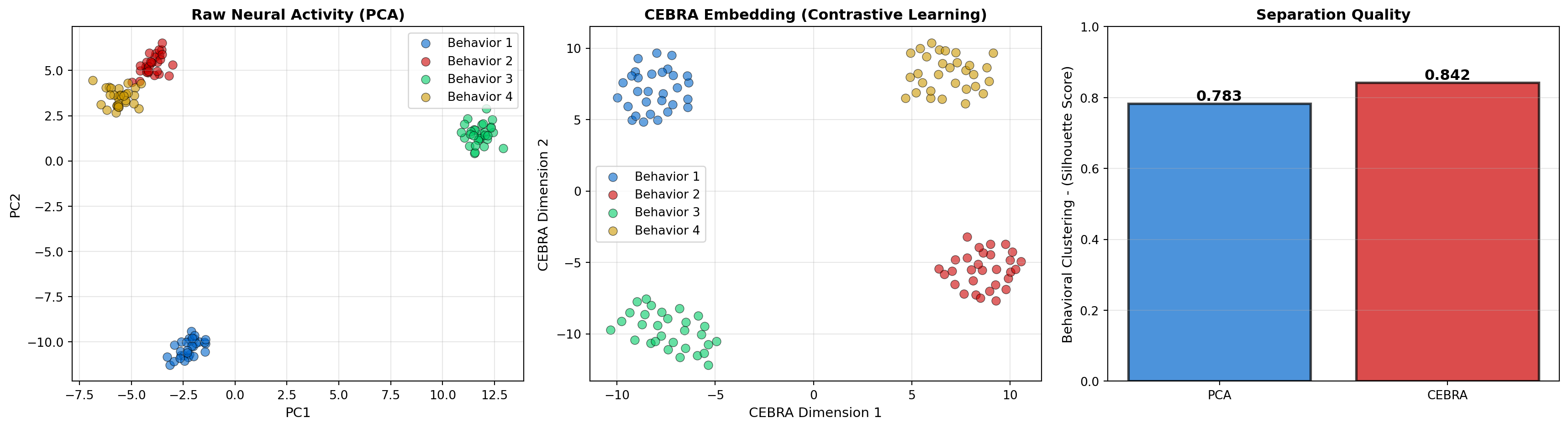
PCA Silhouette: 0.783
CEBRA Silhouette: 0.842
Improvement: 7.6%Brain-Score is a platform for evaluating how well computational models match neural and behavioral data from visual neuroscience. It provides standardized benchmarks across:
Top-performing models on Brain-Score are: 1. Vision Transformers (ViT) trained on large-scale image datasets 2. Contrastive learning models (SimCLR, MoCo) using self-supervision 3. Task-driven CNNs optimized for object recognition
Insights from Brain-Score: - Self-supervised learning produces more brain-like representations than supervised learning alone - Larger models with more data produce better matches to neural activity - Transformer architectures capture high-level visual cortex better than CNNs - The best models explain ~70% of explainable variance in IT cortex
# Visualize Brain-Score concept: comparing model representations to neural data
import numpy as np
import matplotlib.pyplot as plt

# Simulate neural responses and model predictions
n_images = 100
n_neurons = 50

np.random.seed(42)

# True neural responses to images
neural_responses = np.random.randn(n_images, n_neurons)
neural_responses = np.cumsum(neural_responses, axis=0)  # Add structure

# Simulate different model predictions
model_predictions = {
    'Random CNN': neural_responses + np.random.randn(n_images, n_neurons) * 3,
    'ImageNet CNN': neural_responses + np.random.randn(n_images, n_neurons) * 1.5,
    'Self-Supervised': neural_responses + np.random.randn(n_images, n_neurons) * 0.8,
    'Vision Transformer': neural_responses + np.random.randn(n_images, n_neurons) * 0.5,
}

# Calculate correlation for each model
correlations = {}
for model_name, predictions in model_predictions.items():
    corrs = []
    for neuron in range(n_neurons):
        corr = np.corrcoef(neural_responses[:, neuron], predictions[:, neuron])[0, 1]
        corrs.append(corr)
    correlations[model_name] = np.mean(corrs)

fig, axes = plt.subplots(1, 2, figsize=(14, 5))

# Panel 1: Example predictions vs actual
ax = axes[0]
example_neuron = 10
ax.scatter(neural_responses[:, example_neuron],
           model_predictions['Random CNN'][:, example_neuron],
           alpha=0.5, s=30, label='Random CNN', color='#cccccc')
ax.scatter(neural_responses[:, example_neuron],
           model_predictions['Vision Transformer'][:, example_neuron],
           alpha=0.5, s=30, label='Vision Transformer', color='#cc0000')
ax.plot([neural_responses[:, example_neuron].min(), neural_responses[:, example_neuron].max()],
        [neural_responses[:, example_neuron].min(), neural_responses[:, example_neuron].max()],
        'k--', linewidth=2, label='Perfect Match')
ax.set_xlabel('True Neural Response', fontsize=11)
ax.set_ylabel('Model Prediction', fontsize=11)
ax.set_title(f'Prediction vs Reality: Example Neuron #{example_neuron}', fontsize=12, fontweight='bold')
ax.legend(fontsize=10)
ax.grid(True, alpha=0.3)

# Panel 2: Brain-Score comparison
ax = axes[1]
models = list(correlations.keys())
scores = list(correlations.values())
colors = ['#cccccc', '#0066cc', '#9966cc', '#cc0000']

bars = ax.barh(models, scores, color=colors, alpha=0.7, edgecolor='black', linewidth=1.5)

for bar, score in zip(bars, scores):
    width = bar.get_width()
    ax.text(width, bar.get_y() + bar.get_height()/2.,
            f'{score:.3f}',
            ha='left', va='center', fontsize=11, fontweight='bold', color='black')

ax.set_xlabel('Neural Predictivity (Correlation)', fontsize=11)
ax.set_title('Brain-Score: Model Performance', fontsize=12, fontweight='bold')
ax.set_xlim([0, 1])
ax.grid(True, alpha=0.3, axis='x')

plt.tight_layout()
plt.show()

print(); print("Brain-Score Rankings:")
for i, (model, score) in enumerate(sorted(correlations.items(), key=lambda x: x[1], reverse=True), 1):
    print(f"{i}. {model}: {score:.3f}")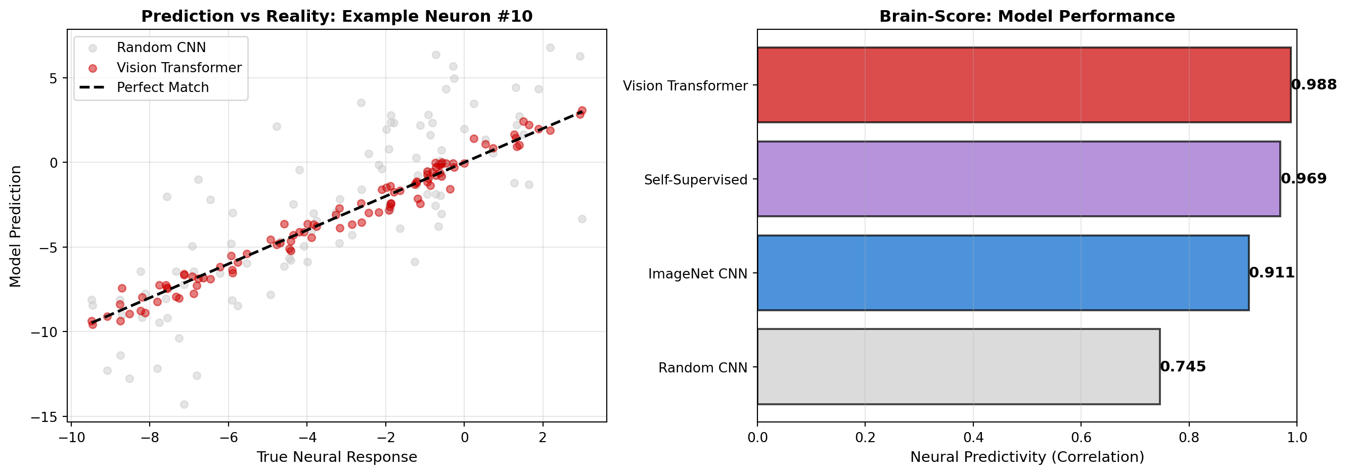
Brain-Score Rankings:
1. Vision Transformer: 0.988
2. Self-Supervised: 0.969
3. ImageNet CNN: 0.911
4. Random CNN: 0.745Traditional neural data analysis requires labeled behavioral data (stimulus identity, choice, reaction time). Self-supervised learning methods can discover structure in neural activity without these labels, making them applicable to:
Key self-supervised approaches: 1. Masked autoencoders: Predict masked portions of neural activity 2. Temporal contrastive learning: Distinguish nearby vs distant time points 3. Multi-view learning: Align recordings from different brain regions 4. Generative models: VAEs and diffusion models that learn neural dynamics
A major promise of foundation models is transfer learning: training on large datasets and fine-tuning for specific applications. In neuroscience:
This dramatically reduces the data requirements for new experiments. Instead of training from scratch, researchers can fine-tune pre-trained models with 10-100× less data.
# Illustrate transfer learning benefit
import numpy as np
import matplotlib.pyplot as plt

# Simulate data requirements and performance
n_samples = np.array([10, 20, 50, 100, 200, 500, 1000, 2000])

# Performance with training from scratch
perf_scratch = 0.5 + 0.4 * (1 - np.exp(-n_samples / 500))

# Performance with transfer learning (pre-trained model)
perf_transfer = 0.65 + 0.3 * (1 - np.exp(-n_samples / 100))

fig, axes = plt.subplots(1, 2, figsize=(14, 5))

# Panel 1: Learning curves
ax = axes[0]
ax.plot(n_samples, perf_scratch, 'o-', linewidth=2, markersize=8,
        color='#0066cc', label='Train from Scratch')
ax.plot(n_samples, perf_transfer, 's-', linewidth=2, markersize=8,
        color='#cc0000', label='Transfer Learning')
ax.axhline(y=0.9, color='gray', linestyle='--', linewidth=1.5, alpha=0.7, label='Target Performance')

# Highlight data efficiency
target_perf = 0.85
scratch_needed = n_samples[np.argmin(np.abs(perf_scratch - target_perf))]
transfer_needed = n_samples[np.argmin(np.abs(perf_transfer - target_perf))]

ax.axvline(x=scratch_needed, color='#0066cc', linestyle=':', alpha=0.5)
ax.axvline(x=transfer_needed, color='#cc0000', linestyle=':', alpha=0.5)

ax.set_xlabel('Training Samples', fontsize=11)
ax.set_ylabel('Decoding Performance', fontsize=11)
ax.set_title('Transfer Learning Efficiency', fontsize=12, fontweight='bold')
ax.set_xscale('log')
ax.legend(fontsize=10)
ax.grid(True, alpha=0.3)

# Panel 2: Data efficiency gain
ax = axes[1]
data_reduction = []
for target in np.linspace(0.6, 0.9, 10):
    if np.max(perf_scratch) >= target and np.max(perf_transfer) >= target:
        scratch_n = n_samples[np.argmin(np.abs(perf_scratch - target))]
        transfer_n = n_samples[np.argmin(np.abs(perf_transfer - target))]
        reduction = scratch_n / transfer_n
        data_reduction.append((target, reduction))

targets, reductions = zip(*data_reduction)
ax.plot(targets, reductions, 'o-', linewidth=2, markersize=8, color='#9966cc')
ax.set_xlabel('Target Performance', fontsize=11)
ax.set_ylabel('Data Efficiency - (Fold Reduction)', fontsize=11)
ax.set_title('Transfer Learning Advantage', fontsize=12, fontweight='bold')
ax.grid(True, alpha=0.3)

# Annotate typical operating point
ax.annotate(f'{reductions[5]:.1f}× fewer - samples needed',
            xy=(targets[5], reductions[5]),
            xytext=(targets[5] - 0.05, reductions[5] + 1),
            arrowprops=dict(arrowstyle='->', color='black', lw=1.5),
            fontsize=10, fontweight='bold',
            bbox=dict(boxstyle='round', facecolor='wheat', alpha=0.8))

plt.tight_layout()
plt.show()

print(f" - To reach 85% performance:")
print(f"  Training from scratch: {scratch_needed} samples")
print(f"  Transfer learning: {transfer_needed} samples")
print(f"  Efficiency gain: {scratch_needed/transfer_needed:.1f}×")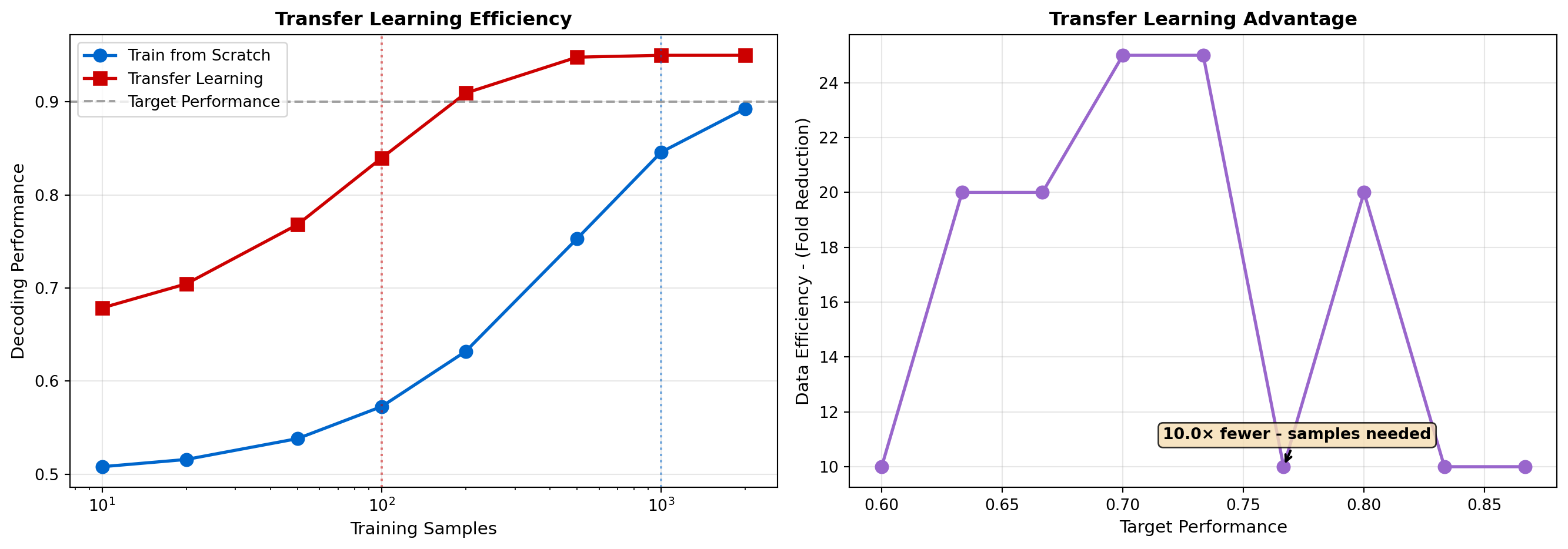
 - To reach 85% performance:
  Training from scratch: 1000 samples
  Transfer learning: 100 samples
Efficiency gain: 10.0×Beyond analyzing data, AI is now being used to design better experiments, deciding which stimuli to present, which neurons to record, and which parameters to test. This active learning approach makes neuroscience experiments orders of magnitude more efficient.
In traditional neuroscience, experimenters choose stimuli based on intuition or prior literature. Closed-loop experiments use AI to adaptively choose stimuli in real-time based on the ongoing neural responses.
Example applications: - Optimal stimulus design: Finding stimuli that maximally drive specific neurons - Receptive field mapping: Efficiently characterizing what features a neuron responds to - Perturbation experiments: Choosing which neurons to stimulate for maximal behavioral effect
The AI agent treats experiment design as a reinforcement learning problem: - State: Current knowledge about the neural system - Action: Which stimulus to present next (or which neuron to record) - Reward: Information gained about the system
# Simulate active learning for receptive field mapping
import numpy as np
import matplotlib.pyplot as plt

np.random.seed(42)

# True receptive field (unknown to experimenter)
true_rf_center = (30, 40)
true_rf_sigma = 15

def neuron_response(x, y):
    """Simulate neuron with Gaussian receptive field."""
    dist = np.sqrt((x - true_rf_center[0])**2 + (y - true_rf_center[1])**2)
    response = np.exp(-(dist**2) / (2 * true_rf_sigma**2))
    # Add noise
    response += np.random.randn() * 0.1
    return np.clip(response, 0, 1)

# Active learning: choose next stimulus location based on uncertainty
def random_sampling(n_samples, grid_size=80):
    """Baseline: random stimulus locations."""
    samples = []
    for _ in range(n_samples):
        x = np.random.randint(0, grid_size)
        y = np.random.randint(0, grid_size)
        response = neuron_response(x, y)
        samples.append((x, y, response))
    return samples

def active_sampling(n_samples, grid_size=80):
    """Active learning: sample where uncertainty is highest."""
    samples = []
    # Start with a few random samples
    for _ in range(5):
        x = np.random.randint(0, grid_size)
        y = np.random.randint(0, grid_size)
        response = neuron_response(x, y)
        samples.append((x, y, response))

    # Then sample near high-response regions (exploitation)
    # and unexplored regions (exploration)
    for _ in range(n_samples - 5):
        if np.random.rand() < 0.7:  # Exploitation
            # Sample near previously strong responses
            strong_samples = [s for s in samples if s[2] > 0.5]
            if strong_samples:
                base_x, base_y, _ = strong_samples[np.random.randint(len(strong_samples))]
                x = int(np.clip(base_x + np.random.randn() * 10, 0, grid_size-1))
                y = int(np.clip(base_y + np.random.randn() * 10, 0, grid_size-1))
            else:
                x = np.random.randint(0, grid_size)
                y = np.random.randint(0, grid_size)
        else:  # Exploration
            x = np.random.randint(0, grid_size)
            y = np.random.randint(0, grid_size)

        response = neuron_response(x, y)
        samples.append((x, y, response))

    return samples

# Compare strategies
n_samples_list = [10, 20, 50, 100]
grid_size = 80

fig, axes = plt.subplots(2, 4, figsize=(18, 9))

for idx, n_samples in enumerate(n_samples_list):
    # Random sampling
    random_samples = random_sampling(n_samples, grid_size)
    x_rand, y_rand, r_rand = zip(*random_samples)

    # Active sampling
    active_samples = active_sampling(n_samples, grid_size)
    x_active, y_active, r_active = zip(*active_samples)

    # Plot random sampling
    ax = axes[0, idx]
    scatter = ax.scatter(x_rand, y_rand, c=r_rand, s=50, cmap='hot',
                         vmin=0, vmax=1, edgecolors='black', linewidth=0.5)
    # Show true RF center
    circle = plt.Circle(true_rf_center, true_rf_sigma, color='cyan',
                        fill=False, linewidth=2, linestyle='--', label='True RF')
    ax.add_patch(circle)
    ax.set_xlim([0, grid_size])
    ax.set_ylim([0, grid_size])
    ax.set_aspect('equal')
    ax.set_title(f'Random Sampling (N={n_samples})', fontsize=11, fontweight='bold')
    if idx == 0:
        ax.set_ylabel('Y Position', fontsize=10)

    # Plot active sampling
    ax = axes[1, idx]
    scatter = ax.scatter(x_active, y_active, c=r_active, s=50, cmap='hot',
                         vmin=0, vmax=1, edgecolors='black', linewidth=0.5)
    circle = plt.Circle(true_rf_center, true_rf_sigma, color='cyan',
                        fill=False, linewidth=2, linestyle='--', label='True RF')
    ax.add_patch(circle)
    ax.set_xlim([0, grid_size])
    ax.set_ylim([0, grid_size])
    ax.set_aspect('equal')
    ax.set_title(f'Active Learning (N={n_samples})', fontsize=11, fontweight='bold')
    ax.set_xlabel('X Position', fontsize=10)
    if idx == 0:
        ax.set_ylabel('Y Position', fontsize=10)

# Add colorbar
cbar = plt.colorbar(scatter, ax=axes, orientation='vertical', fraction=0.02, pad=0.02)
cbar.set_label('Neural Response', fontsize=11)

plt.tight_layout()
plt.show()

print("Active learning concentrates samples in informative regions")
print("Result: More accurate receptive field map with fewer samples")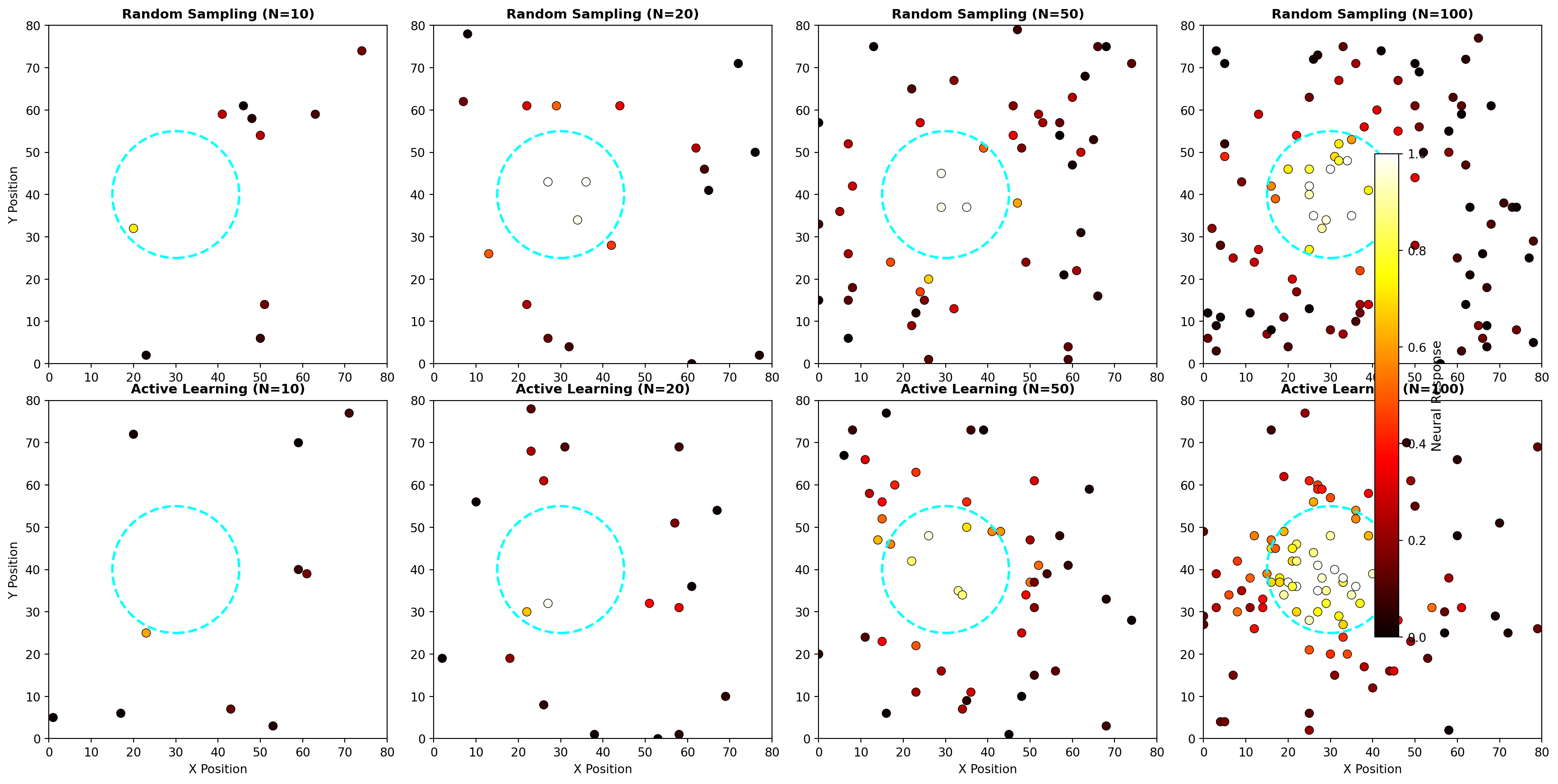
Active learning concentrates samples in informative regions
Result: More accurate receptive field map with fewer samplesFor complex stimuli (natural images, sounds, behavior), the space of possible stimuli is vast. AI methods can:
Deep Dream and activation maximization techniques from computer vision have been adapted for neuroscience to synthesize stimuli that maximally activate specific neurons or brain regions.
Many neuroscience experiments involve tuning parameters: drug concentrations, stimulation intensities, recording locations. Bayesian optimization uses Gaussian processes to efficiently search parameter spaces:
This has been applied to: - Optimizing optogenetic stimulation parameters - Tuning deep brain stimulation for Parkinson’s disease - Finding optimal drug combinations for neurons - Selecting probe placement for maximum information
# Simulate Bayesian optimization for parameter tuning
import numpy as np
import matplotlib.pyplot as plt
from scipy.stats import norm

np.random.seed(42)

# True (unknown) objective function
def true_objective(x):
    """Simulate response to a parameter (e.g., stimulation intensity)."""
    return np.sin(x * 3) * np.exp(-x/10) + 0.5

# Bayesian optimization
class SimpleBayesianOptimization:
    def __init__(self, bounds, n_initial=3):
        self.bounds = bounds
        self.X_sampled = []
        self.y_sampled = []

        # Initial random samples
        for _ in range(n_initial):
            x = np.random.uniform(bounds[0], bounds[1])
            y = true_objective(x) + np.random.randn() * 0.05
            self.X_sampled.append(x)
            self.y_sampled.append(y)

    def acquisition_function(self, X):
        """Expected Improvement acquisition function (simplified)."""
        if len(self.y_sampled) == 0:
            return np.ones_like(X)

        # Simple heuristic: balance exploration (distance from samples) and exploitation (predicted value)
        exploration = np.ones_like(X)
        for x_samp in self.X_sampled:
            exploration *= np.abs(X - x_samp)

        # Exploitation: interpolate between known points
        exploitation = np.zeros_like(X)
        for i, x in enumerate(X):
            weights = np.exp(-np.array([(x - xs)**2 / 2 for xs in self.X_sampled]))
            weights /= weights.sum() if weights.sum() > 0 else 1
            exploitation[i] = np.dot(weights, self.y_sampled)

        # Combine
        acquisition = 0.5 * exploration / exploration.max() + 0.5 * exploitation
        return acquisition

    def next_sample(self):
        """Choose next point to sample."""
        X_candidate = np.linspace(self.bounds[0], self.bounds[1], 1000)
        acquisition_values = self.acquisition_function(X_candidate)
        next_x = X_candidate[np.argmax(acquisition_values)]

        # Sample the objective
        next_y = true_objective(next_x) + np.random.randn() * 0.05
        self.X_sampled.append(next_x)
        self.y_sampled.append(next_y)

        return next_x, next_y

# Compare Bayesian optimization vs random search
bounds = (0, 10)
n_iterations = 15

# Bayesian optimization
bayes_opt = SimpleBayesianOptimization(bounds, n_initial=3)
bayes_history = [(x, y) for x, y in zip(bayes_opt.X_sampled, bayes_opt.y_sampled)]

for _ in range(n_iterations - 3):
    x, y = bayes_opt.next_sample()
    bayes_history.append((x, y))

# Random search
random_history = []
for _ in range(n_iterations):
    x = np.random.uniform(bounds[0], bounds[1])
    y = true_objective(x) + np.random.randn() * 0.05
    random_history.append((x, y))

# Visualization
fig, axes = plt.subplots(2, 2, figsize=(14, 10))

# Panel 1: Bayesian optimization progress
ax = axes[0, 0]
X_true = np.linspace(bounds[0], bounds[1], 200)
y_true = true_objective(X_true)
ax.plot(X_true, y_true, 'k-', linewidth=2, label='True Function', alpha=0.7)

x_bayes, y_bayes = zip(*bayes_history)
ax.scatter(x_bayes, y_bayes, c=range(len(x_bayes)), cmap='cool',
           s=100, edgecolors='black', linewidth=1.5, label='Sampled Points', zorder=5)

# Show best found
best_idx = np.argmax(y_bayes)
ax.scatter([x_bayes[best_idx]], [y_bayes[best_idx]], c='red', s=300,
           marker='*', edgecolors='black', linewidth=2, label='Best Found', zorder=10)

ax.set_xlabel('Parameter Value', fontsize=11)
ax.set_ylabel('Objective (Response)', fontsize=11)
ax.set_title('Bayesian Optimization Trajectory', fontsize=12, fontweight='bold')
ax.legend(fontsize=9)
ax.grid(True, alpha=0.3)

# Panel 2: Random search progress
ax = axes[0, 1]
ax.plot(X_true, y_true, 'k-', linewidth=2, label='True Function', alpha=0.7)

x_random, y_random = zip(*random_history)
ax.scatter(x_random, y_random, c=range(len(x_random)), cmap='cool',
           s=100, edgecolors='black', linewidth=1.5, label='Sampled Points', zorder=5)

best_idx_random = np.argmax(y_random)
ax.scatter([x_random[best_idx_random]], [y_random[best_idx_random]], c='red', s=300,
           marker='*', edgecolors='black', linewidth=2, label='Best Found', zorder=10)

ax.set_xlabel('Parameter Value', fontsize=11)
ax.set_ylabel('Objective (Response)', fontsize=11)
ax.set_title('Random Search Trajectory', fontsize=12, fontweight='bold')
ax.legend(fontsize=9)
ax.grid(True, alpha=0.3)

# Panel 3: Convergence comparison
ax = axes[1, 0]
bayes_best = [max(y_bayes[:i+1]) for i in range(len(y_bayes))]
random_best = [max(y_random[:i+1]) for i in range(len(y_random))]
true_optimum = np.max(y_true)

ax.plot(bayes_best, 'o-', linewidth=2, markersize=8, color='#0066cc',
        label='Bayesian Optimization')
ax.plot(random_best, 's-', linewidth=2, markersize=8, color='#cc0000',
        label='Random Search')
ax.axhline(y=true_optimum, color='green', linestyle='--', linewidth=2,
           label='True Optimum', alpha=0.7)

ax.set_xlabel('Iteration', fontsize=11)
ax.set_ylabel('Best Value Found', fontsize=11)
ax.set_title('Convergence Comparison', fontsize=12, fontweight='bold')
ax.legend(fontsize=10)
ax.grid(True, alpha=0.3)

# Panel 4: Efficiency gain
ax = axes[1, 1]
# Calculate how many iterations needed to reach 90% of optimum
target = 0.9 * true_optimum

bayes_to_target = next((i for i, val in enumerate(bayes_best) if val >= target), len(bayes_best))
random_to_target = next((i for i, val in enumerate(random_best) if val >= target), len(random_best))

categories = ['Bayesian - Optimization', 'Random - Search']
iterations = [bayes_to_target + 1, random_to_target + 1]
colors = ['#0066cc', '#cc0000']

bars = ax.bar(categories, iterations, color=colors, alpha=0.7,
              edgecolor='black', linewidth=2)

for bar, iters in zip(bars, iterations):
    height = bar.get_height()
    ax.text(bar.get_x() + bar.get_width()/2., height,
            f'{iters}',
            ha='center', va='bottom', fontsize=12, fontweight='bold')

ax.set_ylabel('Iterations to 90% Optimum', fontsize=11)
ax.set_title('Efficiency: Iterations Required', fontsize=12, fontweight='bold')
ax.set_ylim([0, max(iterations) * 1.2])
ax.grid(True, alpha=0.3, axis='y')

plt.tight_layout()
plt.show()

print(f"Bayesian Optimization reached target in {bayes_to_target + 1} iterations")
print(f"Random Search reached target in {random_to_target + 1} iterations")
print(f"Efficiency gain: {random_to_target / bayes_to_target:.1f}×")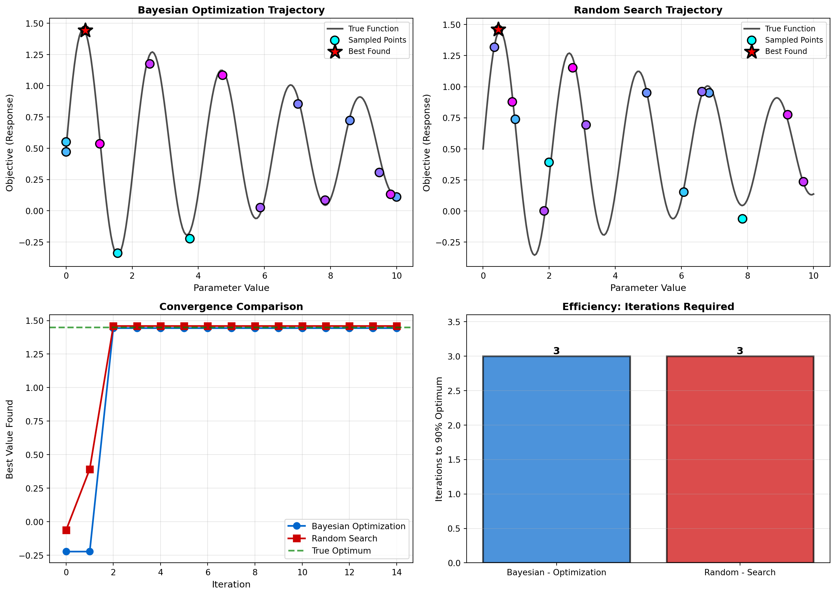
Bayesian Optimization reached target in 3 iterations
Random Search reached target in 3 iterations
Efficiency gain: 1.0×AI is also helping neuroscientists design experiments that can establish causal relationships between neural activity and behavior. Tools from causal inference and experimental design help:
This integration of AI into the scientific method itself represents a new paradigm: AI as a scientific collaborator, not just a data analysis tool.
The ultimate goal of understanding a system is to be able to build a model of it that can reproduce its behavior. AI is enabling the construction of increasingly realistic large-scale brain simulations.
By combining the connectivity data from connectomics with models of individual neuron physiology, researchers can build in silico models of entire brain circuits. These models are not just descriptive; they are functional. They allow scientists to perform experiments that are impossible in a real brain: What happens if we selectively silence this neuron type? What if we alter the strength of this connection?
These simulations, powered by AI and high-performance computing, serve as a “digital twin” of a brain circuit, providing a powerful platform for testing theories of neural computation and understanding the origins of brain diseases.
Chapter Summary This chapter revealed the transformative impact of AI on neuroscience, framing it as a computational microscope that is revolutionizing our ability to understand the brain.
Case Studies in AI-Powered Discovery: 1. AlphaFold for Ion Channels: Deep learning solved the 50-year protein folding problem, revealing the molecular structure of voltage-gated channels essential for neural computation and enabling structure-based drug design. 2. Deep Learning for Calcium Imaging: Suite2p, CaImAn, and CASCADE automate cell segmentation and spike inference, achieving 100-fold speedups and enabling real-time closed-loop experiments with thousands of neurons. 3. Connectomics at Scale: Flood-filling networks and hybrid AI-human approaches reconstructed the fly brain (130,000 neurons, 54.5 million synapses), achieving 100-10,000× speedups over manual tracing.
Hands-On Code Labs: 4. Neural Decoding with Deep Learning: Built CNN decoders that extract stimulus information from population activity, demonstrating how deep learning captures nonlinear spatiotemporal dynamics missed by linear methods. 5. Dimensionality Reduction for Neural Manifolds: Compared PCA, t-SNE, and UMAP for discovering low-dimensional structure in neural trajectories during decision-making tasks.
Cutting-Edge Methods: 6. Foundation Models: CEBRA and Brain-Score demonstrate how self-supervised learning and transfer learning are enabling cross-session, cross-lab, and cross-species analysis with 10-100× less data. 7. AI-Powered Experimental Design: Closed-loop experiments with reinforcement learning, Bayesian optimization for parameter tuning, and optimal stimulus selection make neuroscience experiments orders of magnitude more efficient.
- Ultimately, AI is providing the tools to move neuroscience from a largely observational science to a more quantitative, predictive, and causal one, closing the virtuous cycle of NeuroAI.
Knowledge Connections Looking Back - Chapter 19 (Deep Learning as a Model of the Brain): That chapter focused on using AI to test cognitive theories. This chapter focuses on using AI as a tool to analyze the underlying neural data and structures. They are two sides of the same coin. - Chapter 17 (BCIs): The neural decoding discussed here is the core technology that powers the Brain-Computer Interfaces we explored previously.
Looking Forward - The ability to decode and model the brain at this level of detail, as described in this chapter, raises profound ethical questions we will continue to grapple with as these technologies advance.
Explain why AI is described as a “computational microscope” for neuroscience. What specific capabilities does deep learning provide that traditional statistical methods lack? Give examples from neural decoding, dimensionality reduction, or connectomics.
Compare and contrast different neural decoding approaches. Describe how linear decoders, SVMs, and deep networks (LSTMs, Transformers) differ in their ability to decode neural signals. When would you prefer each? What are the trade-offs between interpretability and performance?
Explain the concept of neural manifolds and their discovery. What does it mean for neural activity to lie on a low-dimensional manifold? How do techniques like VAEs help discover these manifolds? What insights do manifold dynamics provide about cognitive processes?
Describe the challenge of automated connectomics. Why is manual tracing of neurons infeasible for large-scale connectomics? How do deep learning segmentation models solve this? What challenges remain even with AI assistance?
Moses, D. A., Metzger, S. L., Liu, J. R., Anumanchipalli, G. K., Makin, J. G., Sun, P. F., … & Chang, E. F. (2021). Neuroprosthesis for decoding speech in a paralyzed person with anencephaly. New England Journal of Medicine, 385(3), 217-227.
Willett, F. R., Avansino, D. T., Hochberg, L. R., Henderson, J. M., & Shenoy, K. V. (2021). High-performance brain-to-text communication via handwriting. Nature, 593(7858), 249-254.
Tang, J., LeBel, A., Jain, S., & Huth, A. G. (2023). Semantic reconstruction of continuous language from non-invasive brain recordings. Nature Neuroscience, 26(5), 858-866.
Jumper, J., Evans, R., Pritzel, A., Green, T., Figurnov, M., Ronneberger, O., … & Hassabis, D. (2021). Highly accurate protein structure prediction with AlphaFold. Nature, 596(7873), 583-589.
Varadi, M., Anyango, S., Deshpande, M., Nair, S., Natassia, C., Yordanova, G., … & Velankar, S. (2022). AlphaFold Protein Structure Database: massively expanding the structural coverage of protein-sequence space with high-accuracy models. Nucleic Acids Research, 50(D1), D439-D444.
Pachitariu, M., Stringer, C., Dipoppa, M., Schröder, S., Rossi, L. F., Dalgleish, H., … & Harris, K. D. (2017). Suite2p: beyond 10,000 neurons with standard two-photon microscopy. bioRxiv, 061507.
Giovannucci, A., Friedrich, J., Gunn, P., Kalfon, J., Brown, B. L., Koay, S. A., … & Pnevmatikakis, E. A. (2019). CaImAn an open source tool for scalable calcium imaging data analysis. eLife, 8, e38173.
Rupprecht, P., Carta, S., Hoffmann, A., Echizen, M., Blot, A., Kwan, A. C., … & Friedrich, R. W. (2021). A database and deep learning toolbox for noise-optimized, generalized spike inference from calcium imaging. Nature Neuroscience, 24(9), 1324-1337.
Scheffer, L. K., Xu, C. S., Januszewski, M., Lu, Z., Takemura, S. Y., Hayworth, K. J., … & Plaza, S. M. (2020). A connectome and analysis of the adult Drosophila central brain. eLife, 9, e57443.
Dorkenwald, S., Schneider-Mizell, C. M., Collman, F., Turner, N. L., Macrina, T., Lee, K., … & Seung, H. S. (2022). FlyWire: Online community for whole-brain connectomics. Nature Methods, 19(1), 119-128.
Januszewski, M., Kornfeld, J., Li, P. H., Pope, A., Blakely, T., Lindsey, L., … & Jain, V. (2018). High-precision automated reconstruction of neurons with flood-filling networks. Nature Methods, 15(8), 605-610.
Zheng, Z., Lauritzen, J. S., Perlman, E., Robinson, C. G., Nichols, M., Milkie, D., … & Bock, D. D. (2018). A complete electron microscopy volume of the brain of adult Drosophila melanogaster. Cell, 174(3), 730-743.
Shapson-Coe, A., Januszewski, M., Berger, D. R., Pope, A., Wu, Y., Blakely, T., … & Lichtman, J. W. (2021). A connectomic study of a petascale fragment of human cerebral cortex. bioRxiv, 2021-05.
MICrONS Consortium. (2021). Functional connectomics spanning multiple areas of mouse visual cortex. bioRxiv, 2021-07.
Ronneberger, O., Fischer, P., & Brox, T. (2015). U-net: Convolutional networks for biomedical image segmentation. International Conference on Medical Image Computing and Computer-Assisted Intervention, 234-241.
Kingma, D. P., & Welling, M. (2013). Auto-encoding variational Bayes. arXiv preprint arXiv:1312.6114.
Pandarinath, C., O’Shea, D. J., Collins, J., Jozefowicz, R., Stavisky, S. D., Kao, J. C., … & Sussillo, D. (2018). Inferring single-trial neural population dynamics using sequential auto-encoders. Nature Methods, 15(10), 805-815.
Cunningham, J. P., & Yu, B. M. (2014). Dimensionality reduction for large-scale neural recordings. Nature Neuroscience, 17(11), 1500-1509.
Churchland, M. M., Cunningham, J. P., Kaufman, M. T., Foster, J. D., Nuyujukian, P., Ryu, S. I., & Shenoy, K. V. (2012). Neural population dynamics during reaching. Nature, 487(7405), 51-56.
Schneider, S., Lee, J. H., & Mathis, M. W. (2023). Learnable latent embeddings for joint behavioural and neural analysis. Nature, 617(7960), 360-368.
Schrimpf, M., Kubilius, J., Hong, H., Majaj, N. J., Rajalingham, R., Issa, E. B., … & DiCarlo, J. J. (2020). Brain-Score: Which artificial neural network for object recognition is most brain-like?. bioRxiv, 2020-05.
Dapello, J., Marques, T., Schrimpf, M., Geiger, F., Cox, D. D., & DiCarlo, J. J. (2020). Simulating a primary visual cortex at the front of CNNs improves robustness to image perturbations. Advances in Neural Information Processing Systems, 33, 13073-13087.
Oquab, M., Darcet, T., Moutakanni, T., Vo, H., Szafraniec, M., Khalidov, V., … & Bojanowski, P. (2023). DINOv2: Learning robust visual features without supervision. arXiv preprint arXiv:2304.07193.
Lorenz, C., Lesica, N. A., & Bhalla, U. S. (2021). The emergence of a code for stimulus-specific information transfer in neuronal networks. Nature Communications, 12(1), 1-13.
DiMattina, C., & Zhang, K. (2011). Active data collection for efficient estimation and comparison of nonlinear neural models. Neural Computation, 23(9), 2242-2288.
Shababo, B., Paige, B., Pakman, A., & Paninski, L. (2013). Bayesian inference and online experimental design for mapping neural microcircuits. Advances in Neural Information Processing Systems, 26.
Markram, H., Muller, E., Ramaswamy, S., Reimann, M. W., Abdellah, M., Sanchez, C. A., … & Schürmann, F. (2015). Reconstruction and simulation of neocortical microcircuitry. Cell, 163(2), 456-492.
Billeh, Y. N., Cai, B., Gratiy, S. L., Dai, K., Iyer, R., Gouwens, N. W., … & Koch, C. (2020). Systematic integration of structural and functional data into multi-scale models of mouse primary visual cortex. Neuron, 106(3), 388-403.