13 Information Theory Essentials
13.1 7.0 Chapter Goals
Information theory provides essential mathematical tools for quantifying and analyzing information processing in both neural and artificial systems. By the end of this chapter, you should be able to:
- Calculate and interpret fundamental information-theoretic measures like entropy, mutual information, and KL divergence
- Apply information-theoretic analyses to neural data and understand their implications
- Implement efficient coding principles in computational models
- Explain how information theory connects neuroscience and machine learning
- Use Python to compute information measures on various types of data
13.2 7.1 Fundamentals of Information Theory

Claude Shannon’s 1948 paper “A Mathematical Theory of Communication” didn’t just create a new field—it revealed that information itself could be quantified. This insight revolutionized: - Communications: How to send messages efficiently - Computing: How to store and process data - Neuroscience: How brains encode and transmit information - AI: How to measure and optimize learning
The key insight? Information is surprise. A predictable message (“the sun rose today”) carries little information. An unexpected message (“I won the lottery!”) carries much more. Shannon gave us the math to measure this precisely.
Shannon’s Entropy: Quantifying Uncertainty
The central concept in information theory is entropy, which measures the uncertainty or randomness in a probability distribution. For a discrete random variable \(X\) with possible values \(\{x_1, x_2, ..., x_n\}\) and probability mass function \(p(x)\), the entropy \(H(X)\) is defined as:
\[H(X) = -\sum_{i=1}^{n} p(x_i) \log_2 p(x_i)\]
Entropy tells you the minimum average number of yes/no questions needed to identify an outcome: - Coin flip (H = 1 bit): Need 1 question (“Is it heads?”) - Die roll (H ≈ 2.58 bits): Need ~3 questions on average - English letter (H ≈ 4.2 bits): Need ~4-5 questions - Random word from dictionary (H ≈ 11 bits): Need ~11 questions
This is why compression works—most data has less entropy than its raw size suggests. A 1MB text file might compress to 200KB because English text has only ~1 bit of entropy per character, not the 8 bits we use to store it.

Figure 7.1: The binary entropy function showing how uncertainty is maximized at p=0.5 (equal probabilities) and minimized at p=0 or p=1 (complete certainty).
Entropy is measured in bits when using log base 2, and represents the average number of bits needed to encode values of the random variable. A few key properties:
- Entropy is always non-negative
- Entropy is maximized when all outcomes are equally likely
- Entropy is minimized (zero) when one outcome has probability 1
AI Applications: - Model Evaluation: Models with lower entropy predictions are more confident (though not necessarily correct) - Model Compression: Information-theoretic principles guide model pruning and quantization - Learning Algorithms: Maximum entropy methods provide a principled approach to machine learning when knowledge is limited - Feature Selection: High-entropy features typically carry more information for classification tasks
Real-World Applications: - Data Compression: ZIP, JPEG, PNG all rely on entropy coding techniques (Huffman, arithmetic coding) - Cryptography: Secure encryption requires high-entropy (unpredictable) keys - Natural Language Processing: Language models estimate word probabilities and maximize entropy for diverse generation - Neuroscience: Neural spike patterns can be analyzed to determine information content
import numpy as np
import matplotlib.pyplot as plt
from scipy import stats

def entropy(p):
    """Calculate the Shannon entropy of a probability distribution.

    Args:
        p: array of probabilities that sum to 1

    Returns:
        entropy value in bits
    """
    # Remove zeros to avoid log(0) issues
    p = p[p > 0]
    return -np.sum(p * np.log2(p))

    # Example: Calculate entropy of a fair coin toss
p_fair = np.array([0.5, 0.5])
print(f"Entropy of fair coin: {entropy(p_fair):.3f} bits")

    # Example: Calculate entropy of a biased coin toss
p_biased = np.array([0.9, 0.1])
print(f"Entropy of biased coin: {entropy(p_biased):.3f} bits")

    # Visualize entropy for a binary variable as p varies from 0 to 1
p_values = np.linspace(0.001, 0.999, 100)
entropies = [-p*np.log2(p) - (1-p)*np.log2(1-p) for p in p_values]

plt.figure(figsize=(8, 5))
plt.plot(p_values, entropies)
plt.xlabel('Probability of outcome 1')
plt.ylabel('Entropy (bits)')
plt.title('Entropy of a Binary Variable')
plt.axvline(x=0.5, color='r', linestyle='--', alpha=0.3)
plt.grid(True, alpha=0.3)
plt.show()
Joint and Conditional Entropy
For two random variables \(X\) and \(Y\), the joint entropy \(H(X,Y)\) measures the combined uncertainty:
\[H(X,Y) = -\sum_{x \in X} \sum_{y \in Y} p(x,y) \log_2 p(x,y)\]
Conditional entropy \(H(Y|X)\) quantifies the remaining uncertainty in \(Y\) after observing \(X\):
\[H(Y|X) = -\sum_{x \in X} p(x) \sum_{y \in Y} p(y|x) \log_2 p(y|x)\]
The chain rule of entropy relates these concepts:
\[H(X,Y) = H(X) + H(Y|X)\]
Mutual Information: Quantifying Shared Information
Mutual information \(I(X;Y)\) measures the reduction in uncertainty about one variable given knowledge of another:
\[I(X;Y) = H(X) - H(X|Y) = H(Y) - H(Y|X) = H(X) + H(Y) - H(X,Y)\]

Figure 7.2: Venn diagram representation of mutual information as the overlap between entropies of X and Y, showing the relationship between joint, conditional, and marginal entropies.
This symmetric measure ranges from 0 (independent variables) to \(\min(H(X), H(Y))\) (one variable completely determines the other).
AI Applications: - Feature Selection: MI identifies which features provide the most information about target classes - Representation Learning: Maximizing MI between representations and inputs in self-supervised learning (e.g., InfoNCE loss in contrastive learning) - Model Interpretability: MI can measure which neurons/features capture important input attributes - Information Bottleneck: Networks trained to maximize MI with targets while minimizing MI with inputs generalize better
Neuroscience Applications: - Neural Coding: Quantifies how much information spike trains carry about stimuli - Brain Connectivity: Functional connectivity between brain regions can be measured using MI - Sensory Processing: MI helps analyze how sensory information is transformed through neural pathways - Neural Population Decoding: Reveals which groups of neurons collectively encode behaviorally relevant information
def mutual_information(x, y, bins=10):
    """Calculate the mutual information between two continuous variables.

    Args:
        x, y: arrays of observations
        bins: number of bins for discretization

    Returns:
        mutual information value in bits
    """
    # Create joint histogram
    joint_hist, x_edges, y_edges = np.histogram2d(x, y, bins=bins)

    # Normalize to get joint probability
    joint_prob = joint_hist / np.sum(joint_hist)

    # Get marginal probabilities
    x_prob = np.sum(joint_prob, axis=1)
    y_prob = np.sum(joint_prob, axis=0)

    # Calculate mutual information
    mi = 0
    for i in range(bins):
        for j in range(bins):
            if joint_prob[i, j] > 0:
                mi += joint_prob[i, j] * np.log2(joint_prob[i, j] / (x_prob[i] * y_prob[j]))

    return mi

    # Example: Mutual information between correlated variables
np.random.seed(42)
n = 1000
    # Generate correlated data
corr = 0.8
x = np.random.normal(0, 1, n)
y = corr * x + np.sqrt(1 - corr**2) * np.random.normal(0, 1, n)

print(f"Mutual information: {mutual_information(x, y):.3f} bits")

    # Visualize MI for different correlation values
correlation = np.linspace(0, 0.99, 20)
mi_values = []

for c in correlation:
    y_corr = c * x + np.sqrt(1 - c**2) * np.random.normal(0, 1, n)
    mi_values.append(mutual_information(x, y_corr))

plt.figure(figsize=(8, 5))
plt.plot(correlation, mi_values, 'o-')
plt.xlabel('Correlation coefficient')
plt.ylabel('Mutual information (bits)')
plt.title('Mutual Information vs. Correlation')
plt.grid(True, alpha=0.3)
plt.show()
Kullback-Leibler Divergence
The KL divergence \(D_{KL}(P||Q)\) measures how one probability distribution \(P\) differs from a reference distribution \(Q\):
\[D_{KL}(P||Q) = \sum_{i} P(i) \log_2 \frac{P(i)}{Q(i)}\]
Key properties: - KL divergence is always non-negative - \(D_{KL}(P||Q) = 0\) if and only if \(P = Q\) - KL divergence is non-symmetric: \(D_{KL}(P||Q) - eq D_{KL}(Q||P)\)
Think of KL divergence as the “surprise penalty” for using the wrong probability distribution: - If you think it will rain 10% of the time (Q) but it actually rains 50% of the time (P), you’ll be constantly surprised and unprepared - The KL divergence quantifies this total surprise in bits
Asymmetry explained: - \(D_{KL}(P||Q)\): Cost of using Q when truth is P (missing rare events is costly) - \(D_{KL}(Q||P)\): Cost of using P when truth is Q (expecting rare events that don’t happen)
In Machine Learning: - Training neural networks minimizes \(D_{KL}(Data||Model)\) - VAEs minimize \(D_{KL}(Posterior||Prior)\) for regularization - Knowledge distillation uses \(D_{KL}(Teacher||Student)\) to transfer knowledge
A symmetrized version is the Jensen-Shannon divergence:
\[JSD(P||Q) = \frac{1}{2}D_{KL}(P||M) + \frac{1}{2}D_{KL}(Q||M)\]
where \(M = \frac{1}{2}(P + Q)\).
def kl_divergence(p, q):
    """Calculate the KL divergence between two distributions.

    Args:
        p, q: array of probabilities that sum to 1

    Returns:
        KL divergence in bits
    """
    # Filter out zeros to avoid division issues
    mask = (p > 0) & (q > 0)
    p, q = p[mask], q[mask]
    return np.sum(p * np.log2(p / q))

    # Example: KL divergence between Gaussians
x = np.linspace(-5, 5, 1000)
p = stats.norm.pdf(x, 0, 1)  # Standard normal
q = stats.norm.pdf(x, 1, 1.5)  # Shifted and wider normal

    # Normalize to ensure they sum to 1
p = p / np.sum(p)
q = q / np.sum(q)

print(f"KL(P||Q): {kl_divergence(p, q):.3f} bits")
print(f"KL(Q||P): {kl_divergence(q, p):.3f} bits")

    # Visualize
plt.figure(figsize=(8, 5))
plt.plot(x, p, label='P ~ N(0,1)')
plt.plot(x, q, label='Q ~ N(1,1.5)')
plt.xlabel('x')
plt.ylabel('Probability density')
plt.title('KL Divergence Between Distributions')
plt.legend()
plt.grid(True, alpha=0.3)
plt.show()
Channel Capacity
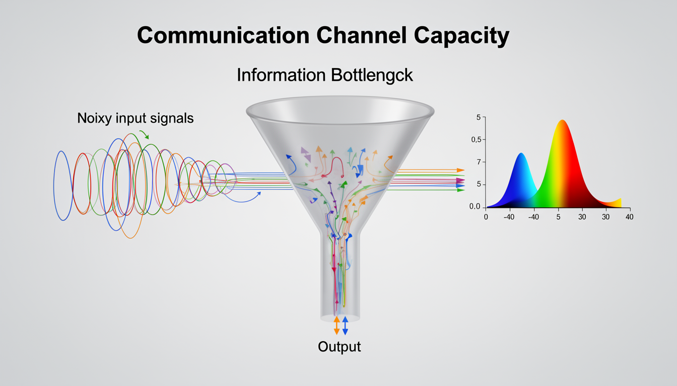
In communication systems, channel capacity represents the maximum rate at which information can be transmitted reliably over a noisy channel. For a discrete memoryless channel, the capacity \(C\) is:
\[C = \max_{p(x)} I(X;Y)\]
where \(p(x)\) is the input distribution. For a Gaussian channel with signal power \(P\) and noise power \(N\), the capacity is:
\[C = \frac{1}{2}\log_2(1 + \frac{P}{N})\]
This concept is crucial in neuroscience for understanding the information-carrying capacity of neural circuits.
Neuroscience Implications: - Neural Bandwidth: Limits how much information a single neuron can transmit (typically 2-3 bits per spike) - Population Coding: Brain overcomes single-neuron capacity limits by distributing information across many neurons - Energy Constraints: Neurons balance information transmission against metabolic costs - Sensory Bottlenecks: Optic nerve’s ~1 million axons create an information bottleneck requiring efficient coding
Engineering Applications: - Communication Systems: Shannon’s capacity theorem revolutionized telecommunications by establishing fundamental limits - 5G Networks: Modern wireless systems approach Shannon capacity with sophisticated coding (LDPC, turbo codes) - Neural Interfaces: Designing optimal neural recording/stimulation devices requires understanding neural channel capacities - AI System Design: Network width and depth choices implicitly reflect channel capacity considerations
13.3 7.2 Neural Coding & Efficiency
Efficient Coding Hypothesis
Proposed by Horace Barlow in the 1960s, the efficient coding hypothesis states that sensory systems have evolved to efficiently represent natural stimuli by reducing redundancy and maximizing information transmission given metabolic constraints.

Figure 7.3: Efficient coding principles in neural systems. The brain adapts to input statistics to create representations that maximize information while minimizing resources through redundancy reduction and sparse coding.
Key principles: - Neurons should encode independent features of the environment - Neural codes should minimize redundancy - Coding strategies should be adapted to the statistics of natural stimuli
Biological Implementations: - Visual System: Retinal ganglion cells adapt to luminance statistics; V1 neurons encode oriented edges (sparse components of natural images) - Auditory System: Cochlear filters adapt to natural sound statistics with 1/f power distributions - Olfactory System: Sparse odor coding with minimal overlapping representations - Adaptation: Sensory neurons dynamically adjust to stimulus statistics to maintain optimal information transmission
AI Applications: - Sparse Autoencoders: Learn efficient, sparse representations similar to V1 receptive fields - Predictive Coding Networks: Optimize to minimize prediction errors, similar to brain’s predictive processing - Model Compression: Pruning, quantization, and knowledge distillation guided by information-theoretic principles - Generative Models: VAEs and diffusion models incorporate information compression principles - Neural Architecture Search: Information Bottleneck principles guide efficient network design
Redundancy Reduction
Natural signals contain statistical regularities and redundancies. Efficient neural coding reduces these redundancies through:
- Decorrelation: Neurons respond to different features, minimizing correlations between their activities
- Predictive coding: Only unpredicted information is transmitted
- Adaptation: Sensory systems adapt to the statistics of their input
The correlation coefficient between two neurons’ activities \(x_i\) and \(x_j\) is:
\[\rho_{ij} = \frac{cov(x_i, x_j)}{\sigma_i \sigma_j}\]
An efficient code would minimize these correlations.
def calculate_neural_correlations(spike_trains):
    """Calculate pairwise correlations between neural spike trains.

    Args:
        spike_trains: array of shape (n_neurons, n_timepoints)

    Returns:
        correlation matrix of shape (n_neurons, n_neurons)
    """
    n_neurons = spike_trains.shape[0]
    correlations = np.zeros((n_neurons, n_neurons))

    for i in range(n_neurons):
        for j in range(n_neurons):
            correlations[i, j] = np.corrcoef(spike_trains[i], spike_trains[j])[0, 1]

    return correlations

    # Simulate some neural data
np.random.seed(42)
n_neurons = 10
n_timepoints = 1000

    # Create correlated spike trains
base = np.random.rand(n_timepoints)
noise_level = 0.3
spike_trains = np.array([base + noise_level * np.random.randn(n_timepoints) for _ in range(n_neurons)])

    # Calculate and visualize correlations
corr_matrix = calculate_neural_correlations(spike_trains)

plt.figure(figsize=(7, 6))
plt.imshow(corr_matrix, cmap='coolwarm', vmin=-1, vmax=1)
plt.colorbar(label='Correlation')
plt.title('Neural Correlation Matrix')
plt.xlabel('Neuron index')
plt.ylabel('Neuron index')
plt.tight_layout()
plt.show()

    # Check average correlation to assess redundancy
print(f"Average pairwise correlation: {np.mean(np.triu(corr_matrix, k=1)):.3f}")
Sparse Coding
Sparse coding aims to represent input data using a small number of active neurons from a large population. This approach:
- Reduces energy consumption (fewer spikes)
- Increases memory capacity
- Facilitates pattern recognition and generalization
The sparseness of a neural code can be measured using the population sparseness metric:
\[S_p = \frac{(\frac{1}{n}\sum_i |r_i|)^2}{\frac{1}{n}\sum_i r_i^2}\]
where \(r_i\) is the response of neuron \(i\), and \(n\) is the number of neurons. \(S_p\) ranges from 0 (dense code) to 1 (maximally sparse).
def calculate_sparseness(population_activity):
    """Calculate population sparseness of neural activity.

    Args:
        population_activity: array of shape (n_neurons, n_samples)

    Returns:
        sparseness values for each sample
    """
    n_samples = population_activity.shape[1]
    sparseness = np.zeros(n_samples)

    for i in range(n_samples):
        r = population_activity[:, i]
        if np.sum(r**2) > 0:  # Avoid division by zero
            sparseness[i] = (np.mean(np.abs(r))**2) / np.mean(r**2)

    return sparseness

    # Simulate neural populations with different levels of sparseness
np.random.seed(42)
n_neurons = 100
n_samples = 10

    # Dense coding (many neurons active)
dense_pop = np.random.rand(n_neurons, n_samples)

    # Sparse coding (few neurons active)
sparse_pop = np.zeros((n_neurons, n_samples))
for i in range(n_samples):
    active_neurons = np.random.choice(n_neurons, size=5, replace=False)
    sparse_pop[active_neurons, i] = np.random.rand(5) * 2

    # Calculate sparseness
dense_sparseness = calculate_sparseness(dense_pop)
sparse_sparseness = calculate_sparseness(sparse_pop)

print(f"Average sparseness (dense): {np.mean(dense_sparseness):.3f}")
print(f"Average sparseness (sparse): {np.mean(sparse_sparseness):.3f}")

    # Visualize
plt.figure(figsize=(12, 5))
plt.subplot(1, 2, 1)
plt.imshow(dense_pop, aspect='auto', cmap='viridis')
plt.title(f'Dense Population - Sparseness: {np.mean(dense_sparseness):.3f}')
plt.xlabel('Sample')
plt.ylabel('Neuron')

plt.subplot(1, 2, 2)
plt.imshow(sparse_pop, aspect='auto', cmap='viridis')
plt.title(f'Sparse Population - Sparseness: {np.mean(sparse_sparseness):.3f}')
plt.xlabel('Sample')
plt.ylabel('Neuron')

plt.tight_layout()
plt.show()
Predictive Coding
Predictive coding posits that neural systems encode and transmit only the “prediction errors” or deviations from expected input, rather than the raw sensory information. This framework:
- Minimizes redundancy by transmitting only what’s unpredicted
- Forms a hierarchical structure where higher levels predict lower levels
- Explains phenomena like sensory adaptation and context effects
Mathematically, if \(y\) is the sensory input and \(\hat{y}\) is the prediction, the prediction error \(e\) is:
\[e = y - \hat{y}\]
Only this error signal is transmitted, allowing for efficient resource use.
13.4 7.3 Information Measures in Neuroscience
Spike Train Information
Neural spike trains carry information through both their rate and timing patterns. To quantify this information, we can:
- Direct method: Estimate the mutual information between stimulus and response directly
- Indirect methods: Use specific information-theoretic quantities like stimulus-specific information
For a spike train response \(r\) to stimulus \(s\), the information transmitted is:
\[I(S;R) = \sum_{s,r} p(s,r) \log_2 \frac{p(s,r)}{p(s)p(r)}\]
This can be decomposed into different coding aspects (rate vs. timing).
def spike_train_information(stimulus, response, bins=10):
    """Calculate mutual information between stimulus and neural response.

    Args:
        stimulus: array of stimulus values
        response: array of neural responses to the stimulus
        bins: number of bins for discretization

    Returns:
        mutual information in bits
    """
    # Discretize continuous variables
    s_bins = np.linspace(min(stimulus), max(stimulus), bins+1)
    r_bins = np.linspace(min(response), max(response), bins+1)

    s_discrete = np.digitize(stimulus, s_bins) - 1
    r_discrete = np.digitize(response, r_bins) - 1

    # Calculate joint and marginal probabilities
    joint_counts = np.zeros((bins, bins))
    for s, r in zip(s_discrete, r_discrete):
        joint_counts[s, r] += 1

    joint_prob = joint_counts / np.sum(joint_counts)
    s_prob = np.sum(joint_prob, axis=1)
    r_prob = np.sum(joint_prob, axis=0)

    # Calculate mutual information
    mi = 0
    for s in range(bins):
        for r in range(bins):
            if joint_prob[s, r] > 0:
                mi += joint_prob[s, r] * np.log2(joint_prob[s, r] / (s_prob[s] * r_prob[r]))

    return mi

    # Simulate neural tuning curves
np.random.seed(42)
n_trials = 1000
stimulus = np.random.uniform(-np.pi, np.pi, n_trials)  # Stimulus orientation

    # Neuron with orientation tuning
preferred_orientation = 0
tuning_width = 0.5

def tuning_curve(stim, preferred, width):
    """Von Mises tuning curve (circular Gaussian)"""
    return np.exp(np.cos(stim - preferred) / width**2) / (2 * np.pi * width**2)

    # Generate noisy neural responses
mean_response = tuning_curve(stimulus, preferred_orientation, tuning_width)
response = np.random.poisson(mean_response * 10)  # Poisson spiking

    # Calculate information
print(f"Stimulus-response information: {spike_train_information(stimulus, response):.3f} bits")

    # Visualize tuning curve
stim_range = np.linspace(-np.pi, np.pi, 100)
tuning = tuning_curve(stim_range, preferred_orientation, tuning_width)

plt.figure(figsize=(10, 5))
plt.subplot(1, 2, 1)
plt.plot(stim_range, tuning)
plt.xlabel('Stimulus orientation (rad)')
plt.ylabel('Mean response')
plt.title('Neural Tuning Curve')

plt.subplot(1, 2, 2)
plt.scatter(stimulus, response, alpha=0.3, s=10)
plt.xlabel('Stimulus orientation (rad)')
plt.ylabel('Spike count')
plt.title('Noisy Neural Responses')

plt.tight_layout()
plt.show()
Neural Decoding Approaches
Neural decoding aims to recover stimulus information from neural activity. Information-theoretic approaches include:
- Maximum likelihood decoding: \(\hat{s} = \arg\max_s p(r|s)\)
- Bayesian decoding: \(p(s|r) \propto p(r|s)p(s)\)
- Population vector decoding: Using the combined activity of a neural population
The decoding accuracy provides a lower bound on the information content of neural activity.
Information Bottleneck Theory
Information bottleneck theory, introduced by Tishby et al., provides a framework for understanding the trade-off between compression and prediction in neural systems. The objective is to find a compressed representation \(T\) of input \(X\) that preserves relevant information about output \(Y\):
\[\min_{p(t|x)} I(X;T) - \beta I(T;Y)\]
where \(\beta\) controls the trade-off between compression \((I(X;T))\) and prediction \((I(T;Y))\).
This has found applications in understanding neural coding and deep learning.
Representational Similarity Analysis
Representational Similarity Analysis (RSA) compares representational geometries between brain regions or between brains and models. The key steps are:
- Compute representational dissimilarity matrices (RDMs) for neural data and models
- Compare these RDMs using correlation or other metrics
The information shared between representations can be quantified using metrics based on KL divergence or mutual information.
13.5 7.4 Noise, Variability & Information
Signal vs Noise in Neural Systems
Neural systems exhibit intrinsic variability that affects information processing:
- Neural variability: Spike count variance often follows Poisson statistics (variance ≈ mean)
- Signal-to-noise ratio (SNR): \(SNR = \frac{\sigma_{signal}^2}{\sigma_{noise}^2}\)
- Fisher information: Measures how well a parameter can be estimated from noisy observations
The Cramér-Rao lower bound states that the variance of any unbiased estimator is at least as high as the inverse of the Fisher information.
def calculate_snr(signal, noise):
    """Calculate signal-to-noise ratio.

    Args:
        signal: array of signal values
        noise: array of noise values

    Returns:
        SNR in decibels
    """
    signal_power = np.mean(signal**2)
    noise_power = np.mean(noise**2)
    snr = 10 * np.log10(signal_power / noise_power)
    return snr

    # Simulate signal with noise
np.random.seed(42)
t = np.linspace(0, 10, 1000)
signal = np.sin(t) + 0.5 * np.sin(3 * t)
noise_levels = [0.1, 0.5, 1.0, 2.0]

plt.figure(figsize=(12, 8))
for i, noise_level in enumerate(noise_levels):
    noise = noise_level * np.random.randn(len(t))
    noisy_signal = signal + noise

    snr = calculate_snr(signal, noise)

    plt.subplot(2, 2, i+1)
    plt.plot(t, signal, 'b-', alpha=0.7, label='Signal')
    plt.plot(t, noisy_signal, 'r-', alpha=0.5, label='Noisy signal')
    plt.title(f'Noise level: {noise_level}, SNR: {snr:.2f} dB')
    plt.xlabel('Time')
    plt.ylabel('Amplitude')
    plt.legend()
    plt.grid(True, alpha=0.3)

plt.tight_layout()
plt.show()
Stochastic Resonance
Stochastic resonance is a counter-intuitive phenomenon where adding noise to a system can enhance signal detection. In neural systems, moderate noise can help weak signals cross thresholds that they wouldn’t reach otherwise.
The information transmission in a system with stochastic resonance follows an inverted U-shape as a function of noise intensity: too little noise doesn’t help, while too much noise overwhelms the signal.
Population Coding Strategies
Neural systems use population coding to improve reliability and increase information content. Key strategies include:
- Redundant coding: Multiple neurons encode similar information
- Distributed coding: Information is spread across many neurons
- Correlation structure: The pattern of correlations affects information content
The information capacity of a population of \(n\) independent neurons can scale linearly with \(n\), but correlations typically reduce this capacity.
def simulate_population_coding(n_neurons, correlation, n_trials=1000):
    """Simulate a population of neurons with specified correlation structure.

    Args:
        n_neurons: number of neurons in the population
        correlation: correlation coefficient between neurons
        n_trials: number of trials to simulate

    Returns:
        population activity matrix of shape (n_neurons, n_trials)
    """
    # Create correlation matrix
    corr_matrix = np.eye(n_neurons)
    corr_matrix[corr_matrix == 0] = correlation

    # Cholesky decomposition to generate correlated Gaussian data
    L = np.linalg.cholesky(corr_matrix)
    uncorrelated = np.random.randn(n_neurons, n_trials)
    population_activity = np.dot(L, uncorrelated)

    return population_activity

    # Simulate populations with different correlation structures
np.random.seed(42)
n_neurons = 20
correlation_levels = [0.0, 0.3, 0.6, 0.9]

plt.figure(figsize=(12, 8))
for i, corr in enumerate(correlation_levels):
    population = simulate_population_coding(n_neurons, corr)

    # Estimate population information capacity
    # Simple approximation based on eigenvalue spectrum of correlation matrix
    corr_matrix = np.corrcoef(population)
    eigenvalues = np.linalg.eigvalsh(corr_matrix)
    information_capacity = np.sum(np.log2(1 + eigenvalues))

    plt.subplot(2, 2, i+1)
    plt.imshow(corr_matrix, cmap='coolwarm', vmin=-1, vmax=1)
    plt.colorbar(label='Correlation')
    plt.title(f'Correlation: {corr} - Info Capacity: {information_capacity:.2f} bits')
    plt.xlabel('Neuron index')
    plt.ylabel('Neuron index')

plt.tight_layout()
plt.show()
Bayesian Inference and Uncertainty
Neural systems appear to implement Bayesian inference, combining prior knowledge with new evidence to form posterior beliefs. Information theory helps quantify uncertainty in these computations through:
- Entropy: Representing overall uncertainty
- KL divergence: Measuring the information gain when updating from prior to posterior
- Mutual information: Quantifying how much new observations reduce uncertainty
The information gained from an observation \(x\) about parameter \(\theta\) is:
\(IG = D_{KL}(p(\theta|x) || p(\theta))\)
13.6 7.5 The Common Currency: Information Theory in Brains and AI
By the end of this chapter, you will be able to:
- Explain the core concepts of information theory, including entropy, mutual information, and KL divergence, using intuitive analogies.
- Calculate these fundamental measures using Python.
- Connect information theory to the brain’s strategies for efficient coding and neural representation.
- Describe how the same information-theoretic principles are used to train and optimize modern AI models.
- Analyze how information flows in both biological and artificial neural networks.
13.7 7.0 Information: The Unifying Language
How can we compare the firing of a neuron to the activation of a unit in a deep neural network? What is the common language that allows us to measure and compare how brains and AI systems process data? The answer is information theory.
Developed by Claude Shannon in 1948 to optimize communication over telegraph lines, information theory provides a universal mathematical framework to quantify uncertainty, communication, and knowledge. It gives us the tools to ask precise questions about any system that processes information, whether it’s made of silicon or cells.
This chapter introduces the core concepts of information theory not as abstract mathematics, but as a practical toolkit for understanding intelligence. We will discover that: - Entropy is a measure of surprise or uncertainty. - Mutual Information quantifies the shared knowledge between two systems. - KL Divergence measures the “cost” of using an imperfect model of the world.
Most importantly, we will see how these concepts form a powerful bridge, revealing that brains and AI are both grappling with the same fundamental challenge: how to efficiently encode, process, and transmit information to make sense of a complex world.
13.8 7.1 The Core Concepts: Quantifying Knowledge and Surprise
Entropy: How Surprising is the News?
Shannon’s core insight was that information is the resolution of uncertainty. A predictable event (the sun rising) carries very little information. An unpredictable event (a lottery win) carries a lot.
Entropy, denoted \(H(X)\), is the measure of this average uncertainty or “surprise” in a system. It is measured in bits.
Entropy tells you the minimum average number of yes/no questions you need to ask to identify an outcome. - A fair coin flip (H=1 bit): You need exactly one question (“Is it heads?”). - A fair eight-sided die (H=3 bits): You need exactly three questions (“Is it > 4?”, “Is it odd?”, etc.). - An English letter (H 248 4.2 bits): You need about 4-5 questions on average.
This is why data compression works. A text file uses 8 bits per character, but since English is predictable, its true entropy is much lower. A ZIP file is just a clever way of re-encoding the data to get closer to its true entropy.
Mathematically, for a set of outcomes with probabilities \(p(x_i)\):
\(H(X) = -\sum_{i} p(x_i) \log_2 p(x_i)\)
Entropy is maximized when all outcomes are equally likely (maximum uncertainty).
Mutual Information: What Do You Know That I Know?
Mutual Information, \(I(X;Y)\), measures the amount of information that one variable tells you about another. It’s the reduction in uncertainty about X after you learn the value of Y.
Imagine two overlapping circles representing the knowledge (entropy) of two people, Alice and Bob. - The area of Alice’s circle is \(H(Alice)\). - The area of Bob’s circle is \(H(Bob)\). - The overlapping area is the Mutual Information, \(I(Alice; Bob)\). It’s the knowledge they share. - The part of Alice’s circle that doesn’t overlap is the Conditional Entropy, \(H(Alice|Bob)\)014what Alice knows that Bob doesn’t.
Figure 7.1: A Venn diagram illustrating the relationship between entropy, conditional entropy, and mutual information.
KL Divergence: The Cost of Using the Wrong Map
Kullback-Leibler (KL) Divergence, \(D_{KL}(P||Q)\), measures how different one probability distribution (\(P\)) is from another (\(Q\)). It’s often used to measure the “cost” or “surprise” of using an approximate model (\(Q\)) when the reality is (\(P\)).
Imagine a tourist has a simplified map of a city (distribution Q), while a local has a perfect map (distribution P). - The KL divergence, \(D_{KL}(P||Q)\), represents the average number of extra questions the tourist has to ask to find their way, because their map is wrong. - It’s not symmetric! \(D_{KL}(P||Q) \u2260 D_{KL}(Q||P)\). The cost of a local using a tourist map is different from the cost of a tourist using a local’s map.
In AI, KL divergence is fundamental. The cross-entropy loss function, used in nearly all classification models, is directly derived from it. Training a model is equivalent to minimizing the KL divergence between the model’s predicted distribution and the true data distribution.
13.9 7.2 The Brain as an Efficient Machine
Why does the brain care about information theory? Because it operates under strict physical and metabolic constraints. It can’t afford to be wasteful. The Efficient Coding Hypothesis, proposed by Horace Barlow, suggests that the brain’s sensory systems have evolved to encode information as efficiently as possible.
This means two things: 1. Reduce Redundancy: Don’t waste energy encoding predictable information. 2. Maximize Information: Transmit the most useful information given the available bandwidth.
How the Brain Achieves Efficiency
- Predictive Coding: The brain seems to be a prediction machine. Higher-level areas constantly generate predictions about incoming sensory information. Only the prediction error014the part of the signal that was not predicted014is sent forward. This is a massively efficient way to reduce redundancy.
- Sparse Coding: Instead of having all neurons firing all the time, the brain uses a sparse code where only a small fraction of neurons are active at any moment. This is incredibly energy-efficient and is a direct inspiration for regularization techniques in AI like dropout and L1 regularization.
The AI Parallel: Compression and Self-Supervised Learning
The brain’s drive for efficiency is mirrored in modern AI. - Autoencoders and VAEs: These architectures are explicitly trained to perform compression. They learn to pass information through a low-dimensional “bottleneck,” forcing them to learn the most efficient, compressed representation of the data. - Contrastive Learning (e.g., SimCLR): A popular self-supervised learning technique where the model learns to maximize the mutual information between two different augmented views of the same image. It’s learning to extract the essential, invariant information, just as the efficient coding hypothesis suggests the brain does.
13.10 7.3 Code Lab: Information Theory in Action
Let’s use Python to calculate these core information-theoretic quantities.
Calculating Entropy and Mutual Information
import numpy as np
import matplotlib.pyplot as plt
from scipy.stats import entropy as scipy_entropy
from sklearn.metrics import mutual_info_score

def entropy_from_counts(counts):
    """Calculate entropy in bits from a list of counts."""
    probs = counts / np.sum(counts)
    return scipy_entropy(probs, base=2)

    # Entropy Example: Fair vs. Biased Die
fair_die_counts = np.array([100, 100, 100, 100, 100, 100])
biased_die_counts = np.array([500, 20, 20, 20, 20, 20])

print(f"Entropy of a fair die: {entropy_from_counts(fair_die_counts):.2f} bits")
print(f"Entropy of a biased die: {entropy_from_counts(biased_die_counts):.2f} bits (less surprise!)")

    # Mutual Information Example: Correlated Variables
np.random.seed(42)
x = np.random.randn(1000)
y = 0.8 * x + np.sqrt(1 - 0.8**2) * np.random.randn(1000)
z = np.random.randn(1000)

    # Discretize for MI calculation
x_bins = np.digitize(x, bins=np.histogram_bin_edges(x, bins=10))
y_bins = np.digitize(y, bins=np.histogram_bin_edges(y, bins=10))
z_bins = np.digitize(z, bins=np.histogram_bin_edges(z, bins=10))

mi_xy = mutual_info_score(x_bins, y_bins)
mi_xz = mutual_info_score(x_bins, z_bins)

print(f"Mutual Information (correlated X, Y): {mi_xy:.2f} bits")
print(f"Mutual Information (uncorrelated X, Z): {mi_xz:.2f} bits")
Calculating KL Divergence
Here we see the “cost” of using a simple model (a standard normal distribution) when the true data comes from a different distribution.
import numpy as np
import matplotlib.pyplot as plt
from scipy.stats import norm

def kl_divergence_continuous(p_samples, q_samples):
    """Estimate KL divergence from samples using binning."""
    # Define shared bins
    min_val = min(p_samples.min(), q_samples.min())
    max_val = max(p_samples.max(), q_samples.max())
    bins = np.linspace(min_val, max_val, 50)

    # Create histograms
    p_hist, _ = np.histogram(p_samples, bins=bins, density=True)
    q_hist, _ = np.histogram(q_samples, bins=bins, density=True)

    # Normalize to get probability distributions
    p_dist = p_hist / p_hist.sum()
    q_dist = q_hist / q_hist.sum()

    # Add small constant to avoid log(0)
    p_dist += 1e-9
    q_dist += 1e-9

    return scipy_entropy(p_dist, q_dist, base=2)

    # KL Divergence Example
    # True distribution P
p_samples = np.random.normal(loc=0.5, scale=1.5, size=10000)
    # Model distribution Q
q_samples = np.random.normal(loc=0, scale=1, size=10000)

kl_pq = kl_divergence_continuous(p_samples, q_samples)

print(f"KL Divergence D_KL(P||Q): {kl_pq:.2f} bits")
print("This is the extra information needed to encode events from P using a code optimized for Q.")

    # Visualization
plt.figure(figsize=(10, 5))
x_axis = np.linspace(-5, 5, 200)
plt.plot(x_axis, norm.pdf(x_axis, 0.5, 1.5), label='True Distribution P')
plt.plot(x_axis, norm.pdf(x_axis, 0, 1), label='Model Distribution Q')
plt.title('KL Divergence Measures the \'Distance\' Between Distributions')
plt.xlabel('Value')
plt.ylabel('Density')
plt.legend()
plt.grid(True, linestyle='--')
plt.show()
13.11 7.4 Information Flow in Networks
Information theory also allows us to measure how information flows through a network, a crucial tool for analyzing both brain circuits and the layers of a deep neural network.
- Transfer Entropy: A powerful measure that can detect directed, causal information flow between two time series. It asks: “Does knowing the past of signal X help me predict the future of signal Y, even after I already know the past of Y?”
- Information Bottleneck: This principle, proposed by Naftali Tishby, suggests that the layers of a deep network act as a series of bottlenecks. Each layer tries to compress the information from the previous layer as much as possible, while still retaining the information that is relevant for the final prediction.
13.12 7.5 Key Takeaways
- Information is the Bridge: Information theory provides a common mathematical language to analyze and compare information processing in brains and AI.
- Brains are Efficient Coders: The brain has evolved powerful strategies like predictive and sparse coding to represent information efficiently, a key source of inspiration for AI.
- AI Training is Information Optimization: Training a neural network can be understood as a process of minimizing the KL divergence (or cross-entropy) between the model’s predictions and the real world.
- Modern AI Relies on Information Principles: Concepts like mutual information and the information bottleneck are not just theoretical; they are at the heart of cutting-edge techniques in self-supervised learning and model compression.
In this chapter, we introduced information theory as the universal currency for understanding intelligent systems.
- We defined the core concepts of entropy (surprise), mutual information (shared knowledge), and KL divergence (the cost of a wrong model), grounding them in intuitive, human-centered analogies.
- We saw how the brain, under metabolic constraints, has evolved to be an efficient information processor, using strategies like predictive and sparse coding to reduce redundancy.
- We drew direct parallels between these biological strategies and modern AI, showing how training a model is equivalent to minimizing KL divergence and how self-supervised learning can be seen as maximizing mutual information.
- Through code examples, we made these abstract concepts tangible, calculating entropy, mutual information, and KL divergence for simple datasets.
By viewing both brains and AI through the lens of information theory, we can see that they are not just analogous; they are both subject to the same fundamental laws governing information, communication, and learning.
13.13 7.5 Exercises
Conceptual Questions
Explain entropy using everyday examples. Describe the entropy of: (a) a fair coin flip, (b) a biased coin with p=0.9, (c) the outcome of rolling a fair die, and (d) picking a random letter from English text. Rank these from highest to lowest entropy and explain your reasoning.
Compare mutual information and correlation. How are mutual information and Pearson correlation similar and different? Can two variables have high mutual information but low correlation? Can they have high correlation but low mutual information? Provide examples.
Explain the efficient coding hypothesis. What does it mean for a neural code to be “efficient”? How do principles like sparse coding and redundancy reduction help achieve efficiency? Why is efficiency important given the brain’s metabolic constraints?
Describe the information bottleneck principle. Explain how deep neural networks can be viewed through the lens of the information bottleneck. What trade-off does each layer make between compression and task-relevant information?
Computational Problems
- Calculate information measures for neural tuning curves. Implement:
- A population of neurons with different preferred orientations (tuning curves)
- Add Poisson noise to their responses
- Calculate the mutual information between stimulus orientation and neural population response
- Compare information from single neurons vs. the population
- Discuss how population coding increases information transmission
- Analyze redundancy in natural images. Using a natural image dataset:
- Calculate pixel-to-pixel correlations
- Compute the entropy of individual pixels vs. the joint entropy of pixel pairs
- Quantify the redundancy using: Redundancy = 1 - H(X,Y) / (H(X) + H(Y))
- Apply whitening (decorrelation) and recalculate redundancy
- Discuss implications for efficient visual coding
- Implement sparse coding. Create:
- A simple sparse autoencoder that learns sparse representations of image patches
- Measure the sparseness of learned representations
- Visualize the learned features and compare them to Gabor filters
- Calculate the coding efficiency (bits per pixel) compared to the original representation
- Measure KL divergence in generative models. Train:
- A simple generative model (e.g., a small variational autoencoder)
- Calculate the KL divergence between the learned latent distribution and the prior
- Plot how KL divergence changes during training
- Experiment with the beta-VAE formulation and see how β affects the KL term and reconstruction quality
Discussion Questions
- Information theory in modern AI architectures. Discuss how information-theoretic principles are used in:
- Self-supervised learning methods like SimCLR (which maximize mutual information)
- Variational autoencoders (which minimize KL divergence)
- Model compression and pruning (which aim to preserve information while reducing parameters)
- Attention mechanisms (which can be viewed as routing information efficiently)
- The efficiency-flexibility trade-off. Highly efficient codes are optimized for specific statistics of their inputs. Discuss:
- What happens when the input statistics change (e.g., the brain encounters a new environment)?
- How might the brain balance efficiency with flexibility to handle novel situations?
- How do AI systems handle this trade-off (e.g., transfer learning, domain adaptation)?
- Could meta-learning algorithms learn to adjust coding strategies based on task demands?
13.14 7.6 References
Shannon, C. E. (1948). A mathematical theory of communication. Bell System Technical Journal, 27(3), 379-423.
Cover, T. M., & Thomas, J. A. (2006). Elements of Information Theory (2nd ed.). Wiley-Interscience.
MacKay, D. J. C. (2003). Information Theory, Inference, and Learning Algorithms. Cambridge University Press.
Rieke, F., Warland, D., de Ruyter van Steveninck, R., & Bialek, W. (1997). Spikes: Exploring the Neural Code. MIT Press.
Barlow, H. B. (1961). Possible principles underlying the transformation of sensory messages. In W. A. Rosenblith (Ed.), Sensory Communication (pp. 217-234). MIT Press.
Fairhall, A. L., Lewen, G. D., Bialek, W., & de Ruyter van Steveninck, R. R. (2001). Efficiency and ambiguity in an adaptive neural code. Nature, 412(6849), 787-792.
Tishby, N., Pereira, F. C., & Bialek, W. (2000). The information bottleneck method. arXiv preprint physics/0004057.
Timme, N. M., & Lapish, C. (2018). A tutorial for information theory in neuroscience. eNeuro, 5(3), ENEURO.0052-18.2018.
Shwartz-Ziv, R., & Tishby, N. (2017). Opening the black box of deep neural networks via information. arXiv preprint arXiv:1703.00810.
Saxe, A. M., Bansal, Y., Dapello, J., Advani, M., Kolchinsky, A., Tracey, B. D., & Cox, D. D. (2019). On the information bottleneck theory of deep learning. Journal of Statistical Mechanics: Theory and Experiment, 2019(12), 124020.
Friston, K. (2010). The free-energy principle: A unified brain theory? Nature Reviews Neuroscience, 11(2), 127-138.
Palmer, S. E., Marre, O., Berry, M. J., & Bialek, W. (2015). Predictive information in a sensory population. Proceedings of the National Academy of Sciences, 112(22), 6908-6913.